Lecture 3 - Deep Learning Tutorial Notebook 1: Introduction to Deep Learning with PyTorch#
Attention
Students are encouraged to use the CSC Mahti platform.
![]()
What we’re going to cover#
This Lecture 3 notebook is strongly based on the PyTorch Computer Vision Tutorial with some modifications to fit our course.
Check out the original PyTorch Computer Vision Tutorial for more details and to see some of the code we won’t be covering in this notebook.
We’re going to cover in this tutorial:
Topic |
Contents |
|---|---|
0. Computer vision libraries in PyTorch |
PyTorch has a bunch of built-in helpful computer vision libraries, let’s check them out. |
1. Load data |
To practice computer vision, we’ll start with some images of different pieces of clothing from FashionMNIST. |
2. Prepare data |
We’ve got some images, let’s load them in with a PyTorch |
3. Model 0: Building a baseline model |
Here we’ll create a multi-class classification model to learn patterns in the data, we’ll also choose a loss function, optimizer and build a training loop. |
4. Making predictions and evaluating model 0 |
Let’s make some predictions with our baseline model and evaluate them. |
5. Setup device agnostic code for future models |
It’s best practice to write device-agnostic code, so let’s set it up. |
6. Model 1: Adding non-linearity |
Experimenting is a large part of machine learning, let’s try and improve upon our baseline model by adding non-linear layers. |
7. Model 2: Convolutional Neural Network (CNN) |
Time to get computer vision specific and introduce the powerful convolutional neural network architecture. |
8. Comparing our models |
We’ve built three different models, let’s compare them. |
9. Evaluating our best model |
Let’s make some predictions on random images and evaluate our best model. |
10. Making a confusion matrix |
A confusion matrix is a great way to evaluate a classification model, let’s see how we can make one. |
11. Saving and loading the best performing model |
Since we might want to use our model later, let’s save it and make sure it loads back in correctly. |
12. Exercise |
10 tasks for you to do on your own to get a deeper insights and understanding of the NNs we have trained. |
0. Setup Libraries and Torchvision#
What are PyTorch and Torchvision?
PyTorch is an open-source ML library from Meta’s AI Research lab. We’ll use it for deep learning, mainly in computer vision.
Torchvision is its companion package for vision work. It ships the common datasets, pretrained model architectures, and image transforms we’ll need.
Let’s import them and check whether we have a GPU available.
# Import PyTorch
import torch
from torch import nn

# Import torchvision
import torchvision
from torchvision import datasets
from torchvision.transforms import ToTensor

# Import matplotlib for visualization
import matplotlib.pyplot as plt

# Check versions
print(
    f"PyTorch version: {torch.__version__}\ntorchvision version: {torchvision.__version__}"
)
PyTorch version: 2.10.0+cu128
torchvision version: 0.25.0+cu128
1. Getting a dataset#
We’re going to use FashionMNIST for this.
MNIST stands for Modified National Institute of Standards and Technology.
The original MNIST dataset contains thousands of examples of handwritten digits (from 0 to 9) and was used to build computer vision models to identify numbers for postal services.
FashionMNIST is made by Zalando Research and is a similar dataset to the original MNIST dataset.
Except it contains grayscale images of 10 different kinds of clothing.
PyTorch bundles this and other standard datasets in torchvision.datasets. You can pull directly from there.
FashionMNIST, the one we use here, is avalible via torchvision.datasets.FashionMNIST().
To download it, we provide the self-explanatory parameters:
root: str- which folder do you want to download the data to?train: Bool- do you want the training or test split?download: Bool- should the data be downloaded?transform: torchvision.transforms- what transformations would you like to do on the data?target_transform- you can transform the targets (labels) if you like too.
Each image in the dataset corresponds to a label from 0-9, representing the ten categories:

# Setup training data
train_data = datasets.FashionMNIST(
    root="data",  # where to download data to?
    train=True,  # get training data
    download=True,  # download data if it doesn't exist on disk
    transform=ToTensor(),  # images come as PIL format, we want to turn into Torch tensors
    target_transform=None,  # you can transform labels as well
)

# Setup testing data
test_data = datasets.FashionMNIST(
    root="data",
    train=False,  # get test data
    download=True,
    transform=ToTensor(),
)
100%|██████████| 26.4M/26.4M [00:01<00:00, 13.3MB/s]
100%|██████████| 29.5k/29.5k [00:00<00:00, 210kB/s]
100%|██████████| 4.42M/4.42M [00:01<00:00, 3.89MB/s]
100%|██████████| 5.15k/5.15k [00:00<00:00, 4.61MB/s]
Let’s look at the first sample in the training data.
# See first training sample
image, label = train_data[0]
image, label
(tensor([[[0.0000, 0.0000, 0.0000, 0.0000, 0.0000, 0.0000, 0.0000, 0.0000,
           0.0000, 0.0000, 0.0000, 0.0000, 0.0000, 0.0000, 0.0000, 0.0000,
           0.0000, 0.0000, 0.0000, 0.0000, 0.0000, 0.0000, 0.0000, 0.0000,
           0.0000, 0.0000, 0.0000, 0.0000],
          [0.0000, 0.0000, 0.0000, 0.0000, 0.0000, 0.0000, 0.0000, 0.0000,
           0.0000, 0.0000, 0.0000, 0.0000, 0.0000, 0.0000, 0.0000, 0.0000,
           0.0000, 0.0000, 0.0000, 0.0000, 0.0000, 0.0000, 0.0000, 0.0000,
           0.0000, 0.0000, 0.0000, 0.0000],
          [0.0000, 0.0000, 0.0000, 0.0000, 0.0000, 0.0000, 0.0000, 0.0000,
           0.0000, 0.0000, 0.0000, 0.0000, 0.0000, 0.0000, 0.0000, 0.0000,
           0.0000, 0.0000, 0.0000, 0.0000, 0.0000, 0.0000, 0.0000, 0.0000,
           0.0000, 0.0000, 0.0000, 0.0000],
          [0.0000, 0.0000, 0.0000, 0.0000, 0.0000, 0.0000, 0.0000, 0.0000,
           0.0000, 0.0000, 0.0000, 0.0000, 0.0039, 0.0000, 0.0000, 0.0510,
           0.2863, 0.0000, 0.0000, 0.0039, 0.0157, 0.0000, 0.0000, 0.0000,
           0.0000, 0.0039, 0.0039, 0.0000],
          [0.0000, 0.0000, 0.0000, 0.0000, 0.0000, 0.0000, 0.0000, 0.0000,
           0.0000, 0.0000, 0.0000, 0.0000, 0.0118, 0.0000, 0.1412, 0.5333,
           0.4980, 0.2431, 0.2118, 0.0000, 0.0000, 0.0000, 0.0039, 0.0118,
           0.0157, 0.0000, 0.0000, 0.0118],
          [0.0000, 0.0000, 0.0000, 0.0000, 0.0000, 0.0000, 0.0000, 0.0000,
           0.0000, 0.0000, 0.0000, 0.0000, 0.0235, 0.0000, 0.4000, 0.8000,
           0.6902, 0.5255, 0.5647, 0.4824, 0.0902, 0.0000, 0.0000, 0.0000,
           0.0000, 0.0471, 0.0392, 0.0000],
          [0.0000, 0.0000, 0.0000, 0.0000, 0.0000, 0.0000, 0.0000, 0.0000,
           0.0000, 0.0000, 0.0000, 0.0000, 0.0000, 0.0000, 0.6078, 0.9255,
           0.8118, 0.6980, 0.4196, 0.6118, 0.6314, 0.4275, 0.2510, 0.0902,
           0.3020, 0.5098, 0.2824, 0.0588],
          [0.0000, 0.0000, 0.0000, 0.0000, 0.0000, 0.0000, 0.0000, 0.0000,
           0.0000, 0.0000, 0.0000, 0.0039, 0.0000, 0.2706, 0.8118, 0.8745,
           0.8549, 0.8471, 0.8471, 0.6392, 0.4980, 0.4745, 0.4784, 0.5725,
           0.5529, 0.3451, 0.6745, 0.2588],
          [0.0000, 0.0000, 0.0000, 0.0000, 0.0000, 0.0000, 0.0000, 0.0000,
           0.0000, 0.0039, 0.0039, 0.0039, 0.0000, 0.7843, 0.9098, 0.9098,
           0.9137, 0.8980, 0.8745, 0.8745, 0.8431, 0.8353, 0.6431, 0.4980,
           0.4824, 0.7686, 0.8980, 0.0000],
          [0.0000, 0.0000, 0.0000, 0.0000, 0.0000, 0.0000, 0.0000, 0.0000,
           0.0000, 0.0000, 0.0000, 0.0000, 0.0000, 0.7176, 0.8824, 0.8471,
           0.8745, 0.8941, 0.9216, 0.8902, 0.8784, 0.8706, 0.8784, 0.8667,
           0.8745, 0.9608, 0.6784, 0.0000],
          [0.0000, 0.0000, 0.0000, 0.0000, 0.0000, 0.0000, 0.0000, 0.0000,
           0.0000, 0.0000, 0.0000, 0.0000, 0.0000, 0.7569, 0.8941, 0.8549,
           0.8353, 0.7765, 0.7059, 0.8314, 0.8235, 0.8275, 0.8353, 0.8745,
           0.8627, 0.9529, 0.7922, 0.0000],
          [0.0000, 0.0000, 0.0000, 0.0000, 0.0000, 0.0000, 0.0000, 0.0000,
           0.0000, 0.0039, 0.0118, 0.0000, 0.0471, 0.8588, 0.8627, 0.8314,
           0.8549, 0.7529, 0.6627, 0.8902, 0.8157, 0.8549, 0.8784, 0.8314,
           0.8863, 0.7725, 0.8196, 0.2039],
          [0.0000, 0.0000, 0.0000, 0.0000, 0.0000, 0.0000, 0.0000, 0.0000,
           0.0000, 0.0000, 0.0235, 0.0000, 0.3882, 0.9569, 0.8706, 0.8627,
           0.8549, 0.7961, 0.7765, 0.8667, 0.8431, 0.8353, 0.8706, 0.8627,
           0.9608, 0.4667, 0.6549, 0.2196],
          [0.0000, 0.0000, 0.0000, 0.0000, 0.0000, 0.0000, 0.0000, 0.0000,
           0.0000, 0.0157, 0.0000, 0.0000, 0.2157, 0.9255, 0.8941, 0.9020,
           0.8941, 0.9412, 0.9098, 0.8353, 0.8549, 0.8745, 0.9176, 0.8510,
           0.8510, 0.8196, 0.3608, 0.0000],
          [0.0000, 0.0000, 0.0039, 0.0157, 0.0235, 0.0275, 0.0078, 0.0000,
           0.0000, 0.0000, 0.0000, 0.0000, 0.9294, 0.8863, 0.8510, 0.8745,
           0.8706, 0.8588, 0.8706, 0.8667, 0.8471, 0.8745, 0.8980, 0.8431,
           0.8549, 1.0000, 0.3020, 0.0000],
          [0.0000, 0.0118, 0.0000, 0.0000, 0.0000, 0.0000, 0.0000, 0.0000,
           0.0000, 0.2431, 0.5686, 0.8000, 0.8941, 0.8118, 0.8353, 0.8667,
           0.8549, 0.8157, 0.8275, 0.8549, 0.8784, 0.8745, 0.8588, 0.8431,
           0.8784, 0.9569, 0.6235, 0.0000],
          [0.0000, 0.0000, 0.0000, 0.0000, 0.0706, 0.1725, 0.3216, 0.4196,
           0.7412, 0.8941, 0.8627, 0.8706, 0.8510, 0.8863, 0.7843, 0.8039,
           0.8275, 0.9020, 0.8784, 0.9176, 0.6902, 0.7373, 0.9804, 0.9725,
           0.9137, 0.9333, 0.8431, 0.0000],
          [0.0000, 0.2235, 0.7333, 0.8157, 0.8784, 0.8667, 0.8784, 0.8157,
           0.8000, 0.8392, 0.8157, 0.8196, 0.7843, 0.6235, 0.9608, 0.7569,
           0.8078, 0.8745, 1.0000, 1.0000, 0.8667, 0.9176, 0.8667, 0.8275,
           0.8627, 0.9098, 0.9647, 0.0000],
          [0.0118, 0.7922, 0.8941, 0.8784, 0.8667, 0.8275, 0.8275, 0.8392,
           0.8039, 0.8039, 0.8039, 0.8627, 0.9412, 0.3137, 0.5882, 1.0000,
           0.8980, 0.8667, 0.7373, 0.6039, 0.7490, 0.8235, 0.8000, 0.8196,
           0.8706, 0.8941, 0.8824, 0.0000],
          [0.3843, 0.9137, 0.7765, 0.8235, 0.8706, 0.8980, 0.8980, 0.9176,
           0.9765, 0.8627, 0.7608, 0.8431, 0.8510, 0.9451, 0.2549, 0.2863,
           0.4157, 0.4588, 0.6588, 0.8588, 0.8667, 0.8431, 0.8510, 0.8745,
           0.8745, 0.8784, 0.8980, 0.1137],
          [0.2941, 0.8000, 0.8314, 0.8000, 0.7569, 0.8039, 0.8275, 0.8824,
           0.8471, 0.7255, 0.7725, 0.8078, 0.7765, 0.8353, 0.9412, 0.7647,
           0.8902, 0.9608, 0.9373, 0.8745, 0.8549, 0.8314, 0.8196, 0.8706,
           0.8627, 0.8667, 0.9020, 0.2627],
          [0.1882, 0.7961, 0.7176, 0.7608, 0.8353, 0.7725, 0.7255, 0.7451,
           0.7608, 0.7529, 0.7922, 0.8392, 0.8588, 0.8667, 0.8627, 0.9255,
           0.8824, 0.8471, 0.7804, 0.8078, 0.7294, 0.7098, 0.6941, 0.6745,
           0.7098, 0.8039, 0.8078, 0.4510],
          [0.0000, 0.4784, 0.8588, 0.7569, 0.7020, 0.6706, 0.7176, 0.7686,
           0.8000, 0.8235, 0.8353, 0.8118, 0.8275, 0.8235, 0.7843, 0.7686,
           0.7608, 0.7490, 0.7647, 0.7490, 0.7765, 0.7529, 0.6902, 0.6118,
           0.6549, 0.6941, 0.8235, 0.3608],
          [0.0000, 0.0000, 0.2902, 0.7412, 0.8314, 0.7490, 0.6863, 0.6745,
           0.6863, 0.7098, 0.7255, 0.7373, 0.7412, 0.7373, 0.7569, 0.7765,
           0.8000, 0.8196, 0.8235, 0.8235, 0.8275, 0.7373, 0.7373, 0.7608,
           0.7529, 0.8471, 0.6667, 0.0000],
          [0.0078, 0.0000, 0.0000, 0.0000, 0.2588, 0.7843, 0.8706, 0.9294,
           0.9373, 0.9490, 0.9647, 0.9529, 0.9569, 0.8667, 0.8627, 0.7569,
           0.7490, 0.7020, 0.7137, 0.7137, 0.7098, 0.6902, 0.6510, 0.6588,
           0.3882, 0.2275, 0.0000, 0.0000],
          [0.0000, 0.0000, 0.0000, 0.0000, 0.0000, 0.0000, 0.0000, 0.1569,
           0.2392, 0.1725, 0.2824, 0.1608, 0.1373, 0.0000, 0.0000, 0.0000,
           0.0000, 0.0000, 0.0000, 0.0000, 0.0000, 0.0000, 0.0000, 0.0000,
           0.0000, 0.0000, 0.0000, 0.0000],
          [0.0000, 0.0000, 0.0000, 0.0000, 0.0000, 0.0000, 0.0000, 0.0000,
           0.0000, 0.0000, 0.0000, 0.0000, 0.0000, 0.0000, 0.0000, 0.0000,
           0.0000, 0.0000, 0.0000, 0.0000, 0.0000, 0.0000, 0.0000, 0.0000,
           0.0000, 0.0000, 0.0000, 0.0000],
          [0.0000, 0.0000, 0.0000, 0.0000, 0.0000, 0.0000, 0.0000, 0.0000,
           0.0000, 0.0000, 0.0000, 0.0000, 0.0000, 0.0000, 0.0000, 0.0000,
           0.0000, 0.0000, 0.0000, 0.0000, 0.0000, 0.0000, 0.0000, 0.0000,
           0.0000, 0.0000, 0.0000, 0.0000]]]),
 9)
1.1 Input and output shapes of a computer vision model#
We’ve got a big tensor of values (the image) and a single value for the target (the label).
Let’s check the image shape:
# What's the shape of the image?
image.shape
torch.Size([1, 28, 28])
The shape of the image tensor is [1, 28, 28] or more specifically:
[color_channels=1, height=28, width=28]
Having color_channels=1 means the image is grayscale.
Different problems will have different input and output shapes, but the idea is the same: turn data into numbers and train a model to find patterns in them.
If color_channels=3, the image comes in pixel values for red, green and blue (this is also known as the RGB color model).
# How many samples are there?
(
    len(train_data.data),
    len(train_data.targets),
    len(test_data.data),
    len(test_data.targets),
)
(60000, 60000, 10000, 10000)
That gives us 60,000 samples for training and 10,000 for testing.
Which classes are in there?
The .classes attribute will tell us.
# See classes
class_names = train_data.classes
class_names
['T-shirt/top',
 'Trouser',
 'Pullover',
 'Dress',
 'Coat',
 'Sandal',
 'Shirt',
 'Sneaker',
 'Bag',
 'Ankle boot']
1.2 Visualizing the data#
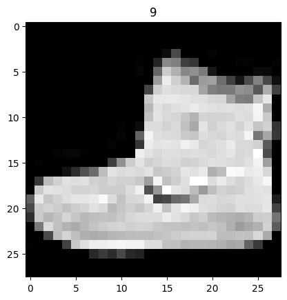
image, label = train_data[0]
print(f"Image shape: {image.shape}")

plt.imshow(
    image.squeeze(), cmap="gray"
)  # image shape is [1, 28, 28] (colour channels, height, width)

plt.title(label)
plt.show()
Image shape: torch.Size([1, 28, 28])
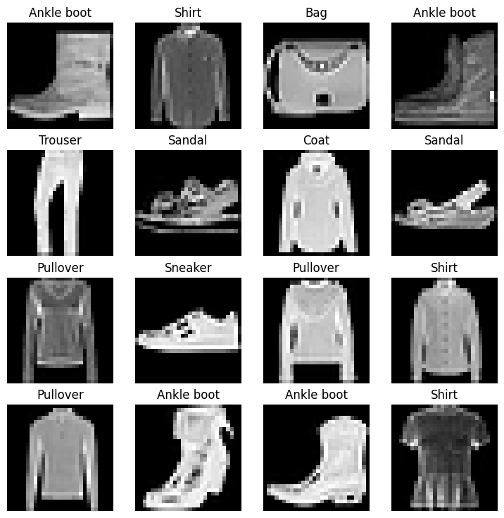
Let’s take a look at a few more images from the dataset:
# Plot more images of the training data
torch.manual_seed(42)
fig = plt.figure(figsize=(9, 9))
rows, cols = 4, 4

for i in range(1, rows * cols + 1):
    random_idx = torch.randint(0, len(train_data), size=[1]).item()
    img, label = train_data[random_idx]
    fig.add_subplot(rows, cols, i)
    plt.imshow(img.squeeze(), cmap="gray")
    plt.title(class_names[label])
    plt.axis(False)
plt.show()
2. Prepare DataLoader#
We’ve got a dataset ready.
The next step is to wrap it in a torch.utils.data.DataLoader (or DataLoader for short).
The DataLoader does roughly what the name suggests: it loads data into a model, both for training and inference.
More specifically, it turns a big Dataset into a Python iterable of smaller chunks called batches (or mini-batches), with the size controlled by the batch_size parameter.
Why do this?
Because it’s more computationally efficient.
In an ideal world you could do the forward pass and backward pass across all of your data at once.
But once you start using really large datasets, unless you’ve got infinite computing power, it’s easier to break them up into batches.
It also gives your model more opportunities to improve.
With mini-batches (small portions of the data), gradient descent is performed more often per epoch (once per mini-batch rather than once per epoch).
So what’s a good batch size?
32 is a reasonable default (Masters & Luschi, 2018) for a lot of problems. It’s a hyperparameter, so we can play with it. Powers of 2 (32, 64, 128, 256, 512) are the usual suspects.
Let’s set up DataLoaders for the training and test sets in the following cells:
from torch.utils.data import DataLoader

# Setup the batch size hyperparameter
BATCH_SIZE = 32

# Turn datasets into iterables (batches)
train_dataloader = DataLoader(
    train_data,  # dataset to turn into iterable
    batch_size=BATCH_SIZE,  # how many samples per batch?
    shuffle=True,  # shuffle data every epoch?
)

test_dataloader = DataLoader(
    test_data,
    batch_size=BATCH_SIZE,
    shuffle=False,  # don't necessarily have to shuffle the testing data
)

# Let's check out what we've created
print(f"Dataloaders: {train_dataloader, test_dataloader} \n")
print(f"Length of train dataloader: {len(train_dataloader)} batches of {BATCH_SIZE}")
print(f"Length of test dataloader: {len(test_dataloader)} batches of {BATCH_SIZE}")
Dataloaders: (<torch.utils.data.dataloader.DataLoader object at 0x7a4fee444f20>, <torch.utils.data.dataloader.DataLoader object at 0x7a4fed7d6c00>)

Length of train dataloader: 1875 batches of 32
Length of test dataloader: 313 batches of 32
# Check out what's inside the training dataloader
train_features_batch, train_labels_batch = next(iter(train_dataloader))
train_features_batch.shape, train_labels_batch.shape
(torch.Size([32, 1, 28, 28]), torch.Size([32]))
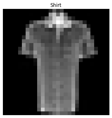
And we can see that the data remains unchanged by checking a single sample.
# Show a sample
torch.manual_seed(42)
random_idx = torch.randint(0, len(train_features_batch), size=[1]).item()
img, label = train_features_batch[random_idx], train_labels_batch[random_idx]
plt.imshow(img.squeeze(), cmap="gray")
plt.title(class_names[label])
plt.axis("Off")
print(f"Image size: {img.shape}")
print(f"Label: {label}, label size: {label.shape}")
Image size: torch.Size([1, 28, 28])
Label: 6, label size: torch.Size([])
3. Model 0: Build a baseline model#
Data is loaded and prepared, so it’s time to build a baseline model by subclassing nn.Module.
A baseline is one of the simplest models we can put together.
We use it as a starting point and try to beat it with more complicated models later on.
Our baseline will consist of two nn.Linear() layers.
Because we’re working with image data, we’re going to use a flatten layer to start things off.
In detail, a nn.Flatten() layer.
nn.Flatten() compresses (“squashes”) the dimensions of a tensor into a single vector.
This is easier to understand when you see it:
# Create a flatten layer
flatten_model = (
    nn.Flatten()
)  # all nn modules function as a model (can do a forward pass)

# Get a single sample
x = train_features_batch[0]

# Flatten the sample
output = flatten_model(x)  # perform forward pass

# Print out what happened
print(f"Shape before flattening: {x.shape} -> [color_channels, height, width]")
print("\n")
print(f"Shape after flattening: {output.shape} -> [color_channels, height*width]")
print("\n")


print(x)  # print the original image tensor
print(output)  # print the flattened image tensor
Shape before flattening: torch.Size([1, 28, 28]) -> [color_channels, height, width]


Shape after flattening: torch.Size([1, 784]) -> [color_channels, height*width]


tensor([[[0.0000, 0.0000, 0.0000, 0.0000, 0.0000, 0.0000, 0.0000, 0.0000,
          0.0000, 0.0000, 0.0000, 0.0000, 0.0000, 0.0000, 0.0000, 0.0000,
          0.0000, 0.0000, 0.0000, 0.0000, 0.0000, 0.0000, 0.0000, 0.0000,
          0.0000, 0.0000, 0.0000, 0.0000],
         [0.0000, 0.0000, 0.0000, 0.0000, 0.0000, 0.0000, 0.0000, 0.0000,
          0.0000, 0.0000, 0.0000, 0.0000, 0.0000, 0.0000, 0.0000, 0.0000,
          0.0000, 0.0000, 0.0000, 0.0000, 0.0000, 0.0000, 0.0000, 0.0000,
          0.0000, 0.0000, 0.0000, 0.0000],
         [0.0000, 0.0000, 0.0000, 0.0000, 0.0000, 0.0000, 0.0000, 0.0000,
          0.0000, 0.0000, 0.0000, 0.0000, 0.0000, 0.0000, 0.0000, 0.0000,
          0.0000, 0.0000, 0.0000, 0.0000, 0.0000, 0.0000, 0.0000, 0.0000,
          0.0000, 0.0000, 0.0000, 0.0000],
         [0.0000, 0.0000, 0.0000, 0.0000, 0.0000, 0.0000, 0.0000, 0.0000,
          0.0000, 0.0039, 0.0039, 0.0000, 0.0000, 0.0078, 0.0078, 0.0000,
          0.0000, 0.0039, 0.0078, 0.0000, 0.0000, 0.0000, 0.0000, 0.0000,
          0.2863, 0.0000, 0.0000, 0.0078],
         [0.0000, 0.0000, 0.0000, 0.0000, 0.0000, 0.0000, 0.0000, 0.0000,
          0.0000, 0.0000, 0.0000, 0.0000, 0.0000, 0.0000, 0.0000, 0.0000,
          0.0000, 0.0000, 0.0000, 0.0000, 0.0000, 0.0000, 0.0000, 0.0000,
          0.3725, 0.0000, 0.0000, 0.0000],
         [0.0000, 0.0000, 0.0000, 0.0000, 0.0000, 0.0000, 0.0000, 0.0000,
          0.0000, 0.0000, 0.0000, 0.0000, 0.0000, 0.3373, 0.3569, 0.2039,
          0.4980, 0.4196, 0.4706, 0.3608, 0.3961, 0.4706, 0.4471, 1.0000,
          0.4314, 0.3451, 0.0078, 0.0000],
         [0.0000, 0.0000, 0.0000, 0.0000, 0.0000, 0.0000, 0.0000, 0.0000,
          0.0000, 0.0000, 0.0000, 0.0000, 0.0000, 0.0706, 0.0824, 0.0706,
          0.4588, 0.4118, 0.4980, 0.2588, 0.2235, 0.2588, 0.0824, 0.0510,
          0.1922, 0.5137, 0.5765, 0.0000],
         [0.0000, 0.0000, 0.0000, 0.0000, 0.0000, 0.0000, 0.0000, 0.0000,
          0.0000, 0.0000, 0.0000, 0.0000, 0.0000, 0.0000, 0.0000, 0.0000,
          0.0000, 0.0000, 0.0000, 0.0000, 0.0000, 0.0000, 0.0000, 0.1333,
          0.8000, 0.5608, 0.5255, 0.2431],
         [0.0000, 0.0000, 0.0000, 0.0000, 0.0000, 0.0000, 0.0000, 0.0000,
          0.0000, 0.0000, 0.0000, 0.0000, 0.0000, 0.0039, 0.0039, 0.0000,
          0.0000, 0.0000, 0.0000, 0.0078, 0.0000, 0.0000, 0.0000, 0.9137,
          0.9686, 0.5137, 0.4353, 0.6471],
         [0.0000, 0.0000, 0.0000, 0.0000, 0.0000, 0.0000, 0.0000, 0.0000,
          0.0000, 0.0000, 0.0000, 0.0000, 0.0000, 0.0000, 0.0000, 0.0000,
          0.0000, 0.0000, 0.0000, 0.0000, 0.0000, 0.0000, 0.0588, 0.3843,
          0.6980, 0.0588, 0.2824, 0.1686],
         [0.0000, 0.0000, 0.0000, 0.0000, 0.0000, 0.0000, 0.0000, 0.0000,
          0.0000, 0.0000, 0.0000, 0.0000, 0.0000, 0.0000, 0.0000, 0.0000,
          0.0000, 0.0000, 0.0000, 0.0000, 0.0000, 0.1333, 0.2078, 0.2157,
          0.6745, 0.2941, 0.1059, 0.0000],
         [0.0000, 0.0000, 0.0000, 0.0000, 0.0000, 0.0000, 0.0000, 0.0000,
          0.0000, 0.0000, 0.0000, 0.0000, 0.0000, 0.0000, 0.0000, 0.0000,
          0.0000, 0.0000, 0.0039, 0.0000, 0.0078, 0.3333, 0.2980, 0.2941,
          0.2039, 0.0314, 0.0000, 0.0000],
         [0.0000, 0.0000, 0.0000, 0.0000, 0.0000, 0.0000, 0.0000, 0.0000,
          0.0000, 0.0000, 0.0000, 0.0000, 0.0000, 0.0000, 0.0000, 0.0000,
          0.0000, 0.0039, 0.0039, 0.0000, 0.2196, 0.5020, 0.0157, 0.0706,
          0.3451, 0.3216, 0.0588, 0.0000],
         [0.0000, 0.0000, 0.0000, 0.0000, 0.0000, 0.0000, 0.0000, 0.0000,
          0.0000, 0.0000, 0.0000, 0.0000, 0.0000, 0.0000, 0.0000, 0.0000,
          0.0000, 0.0000, 0.0000, 0.0157, 0.4863, 0.3843, 0.1804, 0.6235,
          0.7882, 0.6000, 0.1569, 0.0000],
         [0.0000, 0.0000, 0.0000, 0.0000, 0.0000, 0.0000, 0.0000, 0.0000,
          0.0000, 0.0000, 0.0000, 0.0000, 0.0000, 0.0000, 0.0000, 0.0000,
          0.0000, 0.0000, 0.0000, 0.2863, 0.4431, 0.4196, 0.5882, 0.5020,
          0.1020, 0.2235, 0.0549, 0.0000],
         [0.0000, 0.0000, 0.0000, 0.0000, 0.0000, 0.0000, 0.0000, 0.0000,
          0.0000, 0.0000, 0.0000, 0.0000, 0.0000, 0.0000, 0.0000, 0.0000,
          0.0000, 0.0000, 0.0039, 0.4078, 0.4314, 0.7137, 0.1843, 0.2196,
          0.4118, 0.3216, 0.0196, 0.0000],
         [0.0000, 0.0000, 0.0000, 0.0000, 0.0039, 0.0000, 0.0000, 0.0000,
          0.0000, 0.0000, 0.0000, 0.0000, 0.0000, 0.0000, 0.0000, 0.0000,
          0.0000, 0.0000, 0.2549, 0.5647, 0.6275, 0.0824, 0.0000, 0.0000,
          0.5098, 0.3333, 0.0000, 0.0000],
         [0.0000, 0.0000, 0.0000, 0.0000, 0.0000, 0.0000, 0.0039, 0.0039,
          0.0000, 0.0000, 0.0000, 0.0000, 0.0000, 0.0000, 0.0000, 0.0000,
          0.0000, 0.3333, 0.5647, 0.5529, 0.0000, 0.0000, 0.0000, 0.0000,
          0.6510, 0.3059, 0.0000, 0.0000],
         [0.0000, 0.0000, 0.0000, 0.0000, 0.0000, 0.0000, 0.0000, 0.0000,
          0.0000, 0.0000, 0.0000, 0.0000, 0.0000, 0.0000, 0.0000, 0.0000,
          0.1922, 0.7216, 0.4510, 0.0000, 0.0000, 0.0157, 0.0000, 0.0000,
          0.6275, 0.2667, 0.0000, 0.0000],
         [0.0000, 0.0000, 0.0000, 0.0039, 0.0000, 0.0000, 0.0784, 0.0784,
          0.0000, 0.0000, 0.0000, 0.0000, 0.0000, 0.0000, 0.0000, 0.0706,
          0.6392, 0.3804, 0.0000, 0.0000, 0.0000, 0.0314, 0.0000, 0.0000,
          0.6667, 0.1529, 0.0000, 0.0000],
         [0.0000, 0.0000, 0.0039, 0.0000, 0.0314, 0.2471, 0.2980, 0.1686,
          0.0000, 0.0000, 0.0000, 0.0000, 0.0000, 0.0000, 0.0000, 0.5255,
          0.5333, 0.0000, 0.0000, 0.0000, 0.0000, 0.0078, 0.0000, 0.0000,
          0.6784, 0.0706, 0.0000, 0.0039],
         [0.0039, 0.0039, 0.0000, 0.0000, 0.0706, 0.0941, 0.0000, 0.0196,
          0.0000, 0.0000, 0.0000, 0.0000, 0.0000, 0.0000, 0.3451, 0.7137,
          0.0275, 0.0000, 0.0000, 0.0000, 0.0000, 0.0000, 0.0000, 0.0000,
          0.6588, 0.0039, 0.0000, 0.0039],
         [0.0000, 0.0000, 0.0000, 0.0000, 0.0078, 0.1922, 0.1059, 0.1216,
          0.2196, 0.0667, 0.0000, 0.0000, 0.0000, 0.3451, 0.6000, 0.1922,
          0.0000, 0.0196, 0.0000, 0.0039, 0.0000, 0.0000, 0.0000, 0.0000,
          0.6471, 0.0000, 0.0000, 0.0039],
         [0.0510, 0.0275, 0.0000, 0.0000, 0.0000, 0.3294, 0.3804, 0.4000,
          0.4941, 0.3882, 0.0000, 0.0196, 0.5020, 0.6000, 0.2863, 0.0000,
          0.0000, 0.0000, 0.0000, 0.0000, 0.0000, 0.0000, 0.0000, 0.0039,
          0.5451, 0.0000, 0.0000, 0.0000],
         [0.3176, 0.5961, 0.5725, 0.5490, 0.4863, 0.4824, 0.5098, 0.4941,
          0.4431, 0.4431, 0.4471, 0.7216, 0.6235, 0.1647, 0.0000, 0.0000,
          0.0000, 0.0078, 0.0000, 0.0000, 0.0000, 0.0000, 0.0000, 0.0000,
          0.7294, 0.0000, 0.0000, 0.0039],
         [0.0000, 0.0000, 0.0000, 0.0941, 0.1647, 0.1804, 0.2235, 0.2549,
          0.2706, 0.2549, 0.2471, 0.1569, 0.0000, 0.0000, 0.0000, 0.0000,
          0.0000, 0.0000, 0.0000, 0.0000, 0.0000, 0.0000, 0.0000, 0.0000,
          0.7137, 0.0157, 0.0000, 0.0039],
         [0.0000, 0.0000, 0.0000, 0.0000, 0.0000, 0.0000, 0.0000, 0.0000,
          0.0000, 0.0000, 0.0000, 0.0000, 0.0000, 0.0000, 0.0000, 0.0000,
          0.0000, 0.0000, 0.0000, 0.0000, 0.0000, 0.0000, 0.0000, 0.0000,
          0.0000, 0.0000, 0.0000, 0.0000],
         [0.0000, 0.0000, 0.0000, 0.0000, 0.0000, 0.0000, 0.0000, 0.0000,
          0.0000, 0.0000, 0.0000, 0.0000, 0.0000, 0.0000, 0.0000, 0.0000,
          0.0000, 0.0000, 0.0000, 0.0000, 0.0000, 0.0000, 0.0000, 0.0000,
          0.0000, 0.0000, 0.0000, 0.0000]]])
tensor([[0.0000, 0.0000, 0.0000, 0.0000, 0.0000, 0.0000, 0.0000, 0.0000, 0.0000,
         0.0000, 0.0000, 0.0000, 0.0000, 0.0000, 0.0000, 0.0000, 0.0000, 0.0000,
         0.0000, 0.0000, 0.0000, 0.0000, 0.0000, 0.0000, 0.0000, 0.0000, 0.0000,
         0.0000, 0.0000, 0.0000, 0.0000, 0.0000, 0.0000, 0.0000, 0.0000, 0.0000,
         0.0000, 0.0000, 0.0000, 0.0000, 0.0000, 0.0000, 0.0000, 0.0000, 0.0000,
         0.0000, 0.0000, 0.0000, 0.0000, 0.0000, 0.0000, 0.0000, 0.0000, 0.0000,
         0.0000, 0.0000, 0.0000, 0.0000, 0.0000, 0.0000, 0.0000, 0.0000, 0.0000,
         0.0000, 0.0000, 0.0000, 0.0000, 0.0000, 0.0000, 0.0000, 0.0000, 0.0000,
         0.0000, 0.0000, 0.0000, 0.0000, 0.0000, 0.0000, 0.0000, 0.0000, 0.0000,
         0.0000, 0.0000, 0.0000, 0.0000, 0.0000, 0.0000, 0.0000, 0.0000, 0.0000,
         0.0000, 0.0000, 0.0000, 0.0039, 0.0039, 0.0000, 0.0000, 0.0078, 0.0078,
         0.0000, 0.0000, 0.0039, 0.0078, 0.0000, 0.0000, 0.0000, 0.0000, 0.0000,
         0.2863, 0.0000, 0.0000, 0.0078, 0.0000, 0.0000, 0.0000, 0.0000, 0.0000,
         0.0000, 0.0000, 0.0000, 0.0000, 0.0000, 0.0000, 0.0000, 0.0000, 0.0000,
         0.0000, 0.0000, 0.0000, 0.0000, 0.0000, 0.0000, 0.0000, 0.0000, 0.0000,
         0.0000, 0.3725, 0.0000, 0.0000, 0.0000, 0.0000, 0.0000, 0.0000, 0.0000,
         0.0000, 0.0000, 0.0000, 0.0000, 0.0000, 0.0000, 0.0000, 0.0000, 0.0000,
         0.3373, 0.3569, 0.2039, 0.4980, 0.4196, 0.4706, 0.3608, 0.3961, 0.4706,
         0.4471, 1.0000, 0.4314, 0.3451, 0.0078, 0.0000, 0.0000, 0.0000, 0.0000,
         0.0000, 0.0000, 0.0000, 0.0000, 0.0000, 0.0000, 0.0000, 0.0000, 0.0000,
         0.0000, 0.0706, 0.0824, 0.0706, 0.4588, 0.4118, 0.4980, 0.2588, 0.2235,
         0.2588, 0.0824, 0.0510, 0.1922, 0.5137, 0.5765, 0.0000, 0.0000, 0.0000,
         0.0000, 0.0000, 0.0000, 0.0000, 0.0000, 0.0000, 0.0000, 0.0000, 0.0000,
         0.0000, 0.0000, 0.0000, 0.0000, 0.0000, 0.0000, 0.0000, 0.0000, 0.0000,
         0.0000, 0.0000, 0.0000, 0.1333, 0.8000, 0.5608, 0.5255, 0.2431, 0.0000,
         0.0000, 0.0000, 0.0000, 0.0000, 0.0000, 0.0000, 0.0000, 0.0000, 0.0000,
         0.0000, 0.0000, 0.0000, 0.0039, 0.0039, 0.0000, 0.0000, 0.0000, 0.0000,
         0.0078, 0.0000, 0.0000, 0.0000, 0.9137, 0.9686, 0.5137, 0.4353, 0.6471,
         0.0000, 0.0000, 0.0000, 0.0000, 0.0000, 0.0000, 0.0000, 0.0000, 0.0000,
         0.0000, 0.0000, 0.0000, 0.0000, 0.0000, 0.0000, 0.0000, 0.0000, 0.0000,
         0.0000, 0.0000, 0.0000, 0.0000, 0.0588, 0.3843, 0.6980, 0.0588, 0.2824,
         0.1686, 0.0000, 0.0000, 0.0000, 0.0000, 0.0000, 0.0000, 0.0000, 0.0000,
         0.0000, 0.0000, 0.0000, 0.0000, 0.0000, 0.0000, 0.0000, 0.0000, 0.0000,
         0.0000, 0.0000, 0.0000, 0.0000, 0.1333, 0.2078, 0.2157, 0.6745, 0.2941,
         0.1059, 0.0000, 0.0000, 0.0000, 0.0000, 0.0000, 0.0000, 0.0000, 0.0000,
         0.0000, 0.0000, 0.0000, 0.0000, 0.0000, 0.0000, 0.0000, 0.0000, 0.0000,
         0.0000, 0.0000, 0.0039, 0.0000, 0.0078, 0.3333, 0.2980, 0.2941, 0.2039,
         0.0314, 0.0000, 0.0000, 0.0000, 0.0000, 0.0000, 0.0000, 0.0000, 0.0000,
         0.0000, 0.0000, 0.0000, 0.0000, 0.0000, 0.0000, 0.0000, 0.0000, 0.0000,
         0.0000, 0.0000, 0.0039, 0.0039, 0.0000, 0.2196, 0.5020, 0.0157, 0.0706,
         0.3451, 0.3216, 0.0588, 0.0000, 0.0000, 0.0000, 0.0000, 0.0000, 0.0000,
         0.0000, 0.0000, 0.0000, 0.0000, 0.0000, 0.0000, 0.0000, 0.0000, 0.0000,
         0.0000, 0.0000, 0.0000, 0.0000, 0.0000, 0.0157, 0.4863, 0.3843, 0.1804,
         0.6235, 0.7882, 0.6000, 0.1569, 0.0000, 0.0000, 0.0000, 0.0000, 0.0000,
         0.0000, 0.0000, 0.0000, 0.0000, 0.0000, 0.0000, 0.0000, 0.0000, 0.0000,
         0.0000, 0.0000, 0.0000, 0.0000, 0.0000, 0.0000, 0.2863, 0.4431, 0.4196,
         0.5882, 0.5020, 0.1020, 0.2235, 0.0549, 0.0000, 0.0000, 0.0000, 0.0000,
         0.0000, 0.0000, 0.0000, 0.0000, 0.0000, 0.0000, 0.0000, 0.0000, 0.0000,
         0.0000, 0.0000, 0.0000, 0.0000, 0.0000, 0.0000, 0.0039, 0.4078, 0.4314,
         0.7137, 0.1843, 0.2196, 0.4118, 0.3216, 0.0196, 0.0000, 0.0000, 0.0000,
         0.0000, 0.0000, 0.0039, 0.0000, 0.0000, 0.0000, 0.0000, 0.0000, 0.0000,
         0.0000, 0.0000, 0.0000, 0.0000, 0.0000, 0.0000, 0.0000, 0.2549, 0.5647,
         0.6275, 0.0824, 0.0000, 0.0000, 0.5098, 0.3333, 0.0000, 0.0000, 0.0000,
         0.0000, 0.0000, 0.0000, 0.0000, 0.0000, 0.0039, 0.0039, 0.0000, 0.0000,
         0.0000, 0.0000, 0.0000, 0.0000, 0.0000, 0.0000, 0.0000, 0.3333, 0.5647,
         0.5529, 0.0000, 0.0000, 0.0000, 0.0000, 0.6510, 0.3059, 0.0000, 0.0000,
         0.0000, 0.0000, 0.0000, 0.0000, 0.0000, 0.0000, 0.0000, 0.0000, 0.0000,
         0.0000, 0.0000, 0.0000, 0.0000, 0.0000, 0.0000, 0.0000, 0.1922, 0.7216,
         0.4510, 0.0000, 0.0000, 0.0157, 0.0000, 0.0000, 0.6275, 0.2667, 0.0000,
         0.0000, 0.0000, 0.0000, 0.0000, 0.0039, 0.0000, 0.0000, 0.0784, 0.0784,
         0.0000, 0.0000, 0.0000, 0.0000, 0.0000, 0.0000, 0.0000, 0.0706, 0.6392,
         0.3804, 0.0000, 0.0000, 0.0000, 0.0314, 0.0000, 0.0000, 0.6667, 0.1529,
         0.0000, 0.0000, 0.0000, 0.0000, 0.0039, 0.0000, 0.0314, 0.2471, 0.2980,
         0.1686, 0.0000, 0.0000, 0.0000, 0.0000, 0.0000, 0.0000, 0.0000, 0.5255,
         0.5333, 0.0000, 0.0000, 0.0000, 0.0000, 0.0078, 0.0000, 0.0000, 0.6784,
         0.0706, 0.0000, 0.0039, 0.0039, 0.0039, 0.0000, 0.0000, 0.0706, 0.0941,
         0.0000, 0.0196, 0.0000, 0.0000, 0.0000, 0.0000, 0.0000, 0.0000, 0.3451,
         0.7137, 0.0275, 0.0000, 0.0000, 0.0000, 0.0000, 0.0000, 0.0000, 0.0000,
         0.6588, 0.0039, 0.0000, 0.0039, 0.0000, 0.0000, 0.0000, 0.0000, 0.0078,
         0.1922, 0.1059, 0.1216, 0.2196, 0.0667, 0.0000, 0.0000, 0.0000, 0.3451,
         0.6000, 0.1922, 0.0000, 0.0196, 0.0000, 0.0039, 0.0000, 0.0000, 0.0000,
         0.0000, 0.6471, 0.0000, 0.0000, 0.0039, 0.0510, 0.0275, 0.0000, 0.0000,
         0.0000, 0.3294, 0.3804, 0.4000, 0.4941, 0.3882, 0.0000, 0.0196, 0.5020,
         0.6000, 0.2863, 0.0000, 0.0000, 0.0000, 0.0000, 0.0000, 0.0000, 0.0000,
         0.0000, 0.0039, 0.5451, 0.0000, 0.0000, 0.0000, 0.3176, 0.5961, 0.5725,
         0.5490, 0.4863, 0.4824, 0.5098, 0.4941, 0.4431, 0.4431, 0.4471, 0.7216,
         0.6235, 0.1647, 0.0000, 0.0000, 0.0000, 0.0078, 0.0000, 0.0000, 0.0000,
         0.0000, 0.0000, 0.0000, 0.7294, 0.0000, 0.0000, 0.0039, 0.0000, 0.0000,
         0.0000, 0.0941, 0.1647, 0.1804, 0.2235, 0.2549, 0.2706, 0.2549, 0.2471,
         0.1569, 0.0000, 0.0000, 0.0000, 0.0000, 0.0000, 0.0000, 0.0000, 0.0000,
         0.0000, 0.0000, 0.0000, 0.0000, 0.7137, 0.0157, 0.0000, 0.0039, 0.0000,
         0.0000, 0.0000, 0.0000, 0.0000, 0.0000, 0.0000, 0.0000, 0.0000, 0.0000,
         0.0000, 0.0000, 0.0000, 0.0000, 0.0000, 0.0000, 0.0000, 0.0000, 0.0000,
         0.0000, 0.0000, 0.0000, 0.0000, 0.0000, 0.0000, 0.0000, 0.0000, 0.0000,
         0.0000, 0.0000, 0.0000, 0.0000, 0.0000, 0.0000, 0.0000, 0.0000, 0.0000,
         0.0000, 0.0000, 0.0000, 0.0000, 0.0000, 0.0000, 0.0000, 0.0000, 0.0000,
         0.0000, 0.0000, 0.0000, 0.0000, 0.0000, 0.0000, 0.0000, 0.0000, 0.0000,
         0.0000]])
The nn.Flatten() layer took our shape from [color_channels, height, width] to [color_channels, height*width].
Why do that? We’ve turned the pixel data from a 2D grid into one long feature vector, which is the format nn.Linear() layers expect their inputs in.
Let’s build our first model with nn.Flatten() as the opening layer.
from torch import nn


class FashionMNISTModelV0(nn.Module):
    def __init__(self, input_shape: int, hidden_units: int, output_shape: int):
        super().__init__()
        self.layer_stack = nn.Sequential(
            nn.Flatten(),  # neural networks like their inputs in vector form
            nn.Linear(
                in_features=input_shape, out_features=hidden_units
            ),  # in_features = number of features in a data sample (784 pixels)
            nn.Linear(in_features=hidden_units, out_features=output_shape),
        )

    def forward(self, x):
        return self.layer_stack(x)
Now we have got a baseline model class we can use, now let’s instantiate a model.
We’ll need to set the following parameters:
input_shape=784- this is how many features you’ve got going in the model, in our case, it’s one for every pixel in the target image (28 pixels high by 28 pixels wide = 784 features).hidden_units=10- number of units/neurons in the hidden layer(s), this number could be whatever you want but to keep the model small we’ll start with10.output_shape=len(class_names)- since we’re working with a multi-class classification problem, we need an output neuron per class in our dataset.
Let’s create an instance and keep it on the CPU for now.
torch.manual_seed(42)

# Need to setup model with input parameters
model_0 = FashionMNISTModelV0(
    input_shape=784,  # one for every pixel (28x28)
    hidden_units=10,  # how many units in the hidden layer
    output_shape=len(class_names),  # one for every class
)

model_0.to("cpu")  # keep model on CPU to begin with
FashionMNISTModelV0(
  (layer_stack): Sequential(
    (0): Flatten(start_dim=1, end_dim=-1)
    (1): Linear(in_features=784, out_features=10, bias=True)
    (2): Linear(in_features=10, out_features=10, bias=True)
  )
)
3.1 Setup loss, optimizer and evaluation metrics#
Since we’re working on a classification problem, let’s define a accuracy_fn().
# Calculate accuracy (a classification metric)
def accuracy_fn(y_true, y_pred):
    """Calculates accuracy between truth labels and predictions.

    Args:
        y_true (torch.Tensor): Truth labels for predictions.
        y_pred (torch.Tensor): Predictions to be compared to predictions.

    Returns:
        [torch.float]: Accuracy value between y_true and y_pred, e.g. 78.45
    """
    correct = torch.eq(y_true, y_pred).sum().item()
    acc = (correct / len(y_pred)) * 100
    return acc


# Setup loss function and optimizer
loss_fn = (
    nn.CrossEntropyLoss()
)  # this is also called "criterion"/"cost function" in some places

optimizer = torch.optim.SGD(params=model_0.parameters(), lr=0.1)
3.2 Creating a function to time our experiments#
Loss function and optimizer are ready, so we can start training.
But let’s add a small experiment along the way: a timing function to measure how long the model takes to train on CPU versus GPU. We’ll train this one on CPU and the next on GPU, then compare.
We’ll train this model on the CPU but the next one on the GPU and see what happens.
Our timing function will import the timeit.default_timer() function from the Python timeit module.
from timeit import default_timer as timer


def print_train_time(start: float, end: float, device: torch.device = None):
    """Prints difference between start and end time.

    Args:
        start (float): Start time of computation (preferred in timeit format).
        end (float): End time of computation.
        device ([type], optional): Device that compute is running on. Defaults to None.

    Returns:
        float: time between start and end in seconds (higher is longer).
    """
    total_time = end - start
    print(f"Train time on {device}: {total_time:.3f} seconds")
    return total_time
3.3 Creating a training loop and training a model on batches of data#
We’ve got all the pieces in place: a timer, loss function, optimizer, model, and (most importantly) some data. Time to write the training and testing loops.
Since our data is in batch form, we’ll loop through the batches inside train_dataloader and test_dataloader. Each batch holds BATCH_SIZE samples of X (features) and y (labels) — with BATCH_SIZE=32, that’s 32 images and labels per batch.
Because we’re working batch by batch, loss and accuracy get calculated per batch, so we’ll average them out by dividing by the number of batches in each dataloader at the end.
Here’s the plan:
Loop through epochs.
Loop through training batches, run training steps, calculate train loss per batch.
Loop through testing batches, run testing steps, calculate test loss per batch.
Print what’s going on.
Time the whole thing (for fun).
# Import tqdm for progress bar
from tqdm.auto import tqdm

# Set the seed and start the timer
torch.manual_seed(42)
train_time_start_on_cpu = timer()

# Set the number of epochs (we'll keep this small for faster training times)
epochs = 3

# Create training and testing loop
for epoch in tqdm(range(epochs)):
    print(f"Epoch: {epoch}\n-------")
    ### Training
    train_loss = 0
    # Add a loop to loop through training batches
    for batch, (X, y) in enumerate(train_dataloader):
        model_0.train()
        # 1. Forward pass
        y_pred = model_0(X)

        # 2. Calculate loss (per batch)
        loss = loss_fn(y_pred, y)
        train_loss += loss  # accumulatively add up the loss per epoch

        # 3. Optimizer zero grad
        optimizer.zero_grad()

        # 4. Loss backward
        loss.backward()

        # 5. Optimizer step
        optimizer.step()

        # Print out how many samples have been seen
        if batch % 400 == 0:
            print(f"Looked at {batch * len(X)}/{len(train_dataloader.dataset)} samples")

    # Divide total train loss by length of train dataloader (average loss per batch per epoch)
    train_loss /= len(train_dataloader)

    ### Testing
    # Setup variables for accumulatively adding up loss and accuracy
    test_loss, test_acc = 0, 0
    model_0.eval()
    with torch.inference_mode():
        for X, y in test_dataloader:
            # 1. Forward pass
            test_pred = model_0(X)

            # 2. Calculate loss (accumulatively)
            test_loss += loss_fn(
                test_pred, y
            )  # accumulatively add up the loss per epoch

            # 3. Calculate accuracy (preds need to be same as y_true)
            test_acc += accuracy_fn(y_true=y, y_pred=test_pred.argmax(dim=1))

        # Calculations on test metrics need to happen inside torch.inference_mode()
        # Divide total test loss by length of test dataloader (per batch)
        test_loss /= len(test_dataloader)

        # Divide total accuracy by length of test dataloader (per batch)
        test_acc /= len(test_dataloader)

    ## Print out what's happening
    print(
        f"\nTrain loss: {train_loss:.5f} | Test loss: {test_loss:.5f}, Test acc: {test_acc:.2f}%\n"
    )

# Calculate training time
train_time_end_on_cpu = timer()
total_train_time_model_0 = print_train_time(
    start=train_time_start_on_cpu,
    end=train_time_end_on_cpu,
    device=str(next(model_0.parameters()).device),
)
Epoch: 0
-------
Looked at 0/60000 samples
Looked at 12800/60000 samples
Looked at 25600/60000 samples
Looked at 38400/60000 samples
Looked at 51200/60000 samples

Train loss: 0.59039 | Test loss: 0.50954, Test acc: 82.04%

Epoch: 1
-------
Looked at 0/60000 samples
Looked at 12800/60000 samples
Looked at 25600/60000 samples
Looked at 38400/60000 samples
Looked at 51200/60000 samples

Train loss: 0.47633 | Test loss: 0.47989, Test acc: 83.20%

Epoch: 2
-------
Looked at 0/60000 samples
Looked at 12800/60000 samples
Looked at 25600/60000 samples
Looked at 38400/60000 samples
Looked at 51200/60000 samples

Train loss: 0.45503 | Test loss: 0.47664, Test acc: 83.43%

Train time on cpu: 28.764 seconds
Our baseline model did fairly well.
It didn’t take too long to train either, even just on the CPU, I wonder if it’ll speed up on the GPU?
Let’s write some code to evaluate our model.
4. Make predictions and get Model 0 results#
Since we’ll be building a few models, it makes sense to write some code that evaluates them all the same way.
Let’s create a function that takes a trained model, a DataLoader, a loss function, and an accuracy function.
It’ll run predictions on the data in the DataLoader and score them using the loss and accuracy functions.
torch.manual_seed(42)


def eval_model(
    model: torch.nn.Module,
    data_loader: torch.utils.data.DataLoader,
    loss_fn: torch.nn.Module,
    accuracy_fn,
):
    """Returns a dictionary containing the results of model predicting on data_loader.

    Args:
        model (torch.nn.Module): A PyTorch model capable of making predictions on data_loader.
        data_loader (torch.utils.data.DataLoader): The target dataset to predict on.
        loss_fn (torch.nn.Module): The loss function of model.
        accuracy_fn: An accuracy function to compare the models predictions to the truth labels.

    Returns:
        (dict): Results of model making predictions on data_loader.
    """
    loss, acc = 0, 0
    model.eval()
    with torch.inference_mode():
        for X, y in data_loader:
            # Make predictions with the model
            y_pred = model(X)

            # Accumulate the loss and accuracy values per batch
            loss += loss_fn(y_pred, y)
            acc += accuracy_fn(
                y_true=y, y_pred=y_pred.argmax(dim=1)
            )  # For accuracy, need the prediction labels (logits -> pred_prob -> pred_labels)

        # Scale loss and acc to find the average loss/acc per batch
        loss /= len(data_loader)
        acc /= len(data_loader)

    return {
        "model_name": model.__class__.__name__,  # only works when model was created with a class
        "model_loss": loss.item(),
        "model_acc": acc,
    }


# Calculate model 0 results on test dataset
model_0_results = eval_model(
    model=model_0, data_loader=test_dataloader, loss_fn=loss_fn, accuracy_fn=accuracy_fn
)
model_0_results
{'model_name': 'FashionMNISTModelV0',
 'model_loss': 0.47663888335227966,
 'model_acc': 83.42651757188499}
We can use this dictionary to compare the baseline model results to other models later on.
5. Setup device agnostic-code (for using a GPU if there is one)#
We’ve seen how long it takes to train ma PyTorch model on 60,000 samples on CPU.
But keep in mind:
Model training time is dependent on hardware used.
Generally, more processors means faster training and smaller models on smaller datasets will often train faster than large models and large datasets.
Now let’s setup some device-agnostic code for our models and data to run on GPU if it’s available.
If you’re running this notebook on Google Colab, and you don’t have a GPU turned on yet, it’s now time to turn one on via Runtime -> Change runtime type -> Hardware accelerator -> GPU.
If you do this, your runtime will likely reset and you’ll have to run all of the cells above by going Runtime -> Run before.
# Setup device agnostic code
import torch

device = "cuda" if torch.cuda.is_available() else "cpu"
device
'cuda'
6. Model 1: Building a better model with non-linearity#
We’ll recreating a similar model to before, except this time we’ll put non-linear functions (nn.ReLU()) in between each linear layer.
Do non-linear functions benefit our model?
# Create a model with non-linear and linear layers
class FashionMNISTModelV1(nn.Module):
    def __init__(self, input_shape: int, hidden_units: int, output_shape: int):
        super().__init__()
        self.layer_stack = nn.Sequential(
            nn.Flatten(),  # flatten inputs into single vector
            nn.Linear(in_features=input_shape, out_features=hidden_units),
            nn.ReLU(),
            nn.Linear(in_features=hidden_units, out_features=output_shape),
            nn.ReLU(),
        )

    def forward(self, x: torch.Tensor):
        return self.layer_stack(x)
Now let’s instantiate it with the same settings as before: input_shape=784 (the number of features in our image data), hidden_units=10 (small, matching the baseline), and output_shape=len(class_names) (one output unit per class).
Note: Most settings are unchanged from the baseline. The only difference is the added non-linear layers. That’s standard practice when running ML experiments: change one thing, see what happens, repeat.
torch.manual_seed(42)

model_1 = FashionMNISTModelV1(
    input_shape=784,  # number of input features
    hidden_units=10,
    output_shape=len(class_names),  # number of output classes desired
).to(device)  # send model to GPU if it's available

next(model_1.parameters()).device  # check model device
device(type='cuda', index=0)
6.1 Setup loss, optimizer and evaluation metrics#
As usual, we’ll setup a loss function, an optimizer and an evaluation metric
# Setup loss, optimizer and evaluation metrics
loss_fn = nn.CrossEntropyLoss()
optimizer = torch.optim.SGD(params=model_1.parameters(), lr=0.1)
6.2 Functionizing training and test loops#
So far we’ve been writing train and test loops over and over.
Let’s write them again but this time we’ll put them in functions so they can be called again and again.
Since we’re using device-agnostic code now, we’ll make sure to call .to(device) on the feature (X) and target (y) tensors.
For the training loop we’ll create a function called train_step() which takes in a model, a DataLoader a loss function and an optimizer.
The testing loop will be similar but it’ll be called test_step() and it’ll take in a model, a DataLoader, a loss function and an evaluation function.
def train_step(
    model: torch.nn.Module,
    data_loader: torch.utils.data.DataLoader,
    loss_fn: torch.nn.Module,
    optimizer: torch.optim.Optimizer,
    accuracy_fn,
    device: torch.device = device,
):
    train_loss, train_acc = 0, 0
    model.to(device)
    for batch, (X, y) in enumerate(data_loader):
        # Send data to GPU
        X, y = X.to(device), y.to(device)

        # 1. Forward pass
        y_pred = model(X)

        # 2. Calculate loss
        loss = loss_fn(y_pred, y)
        train_loss += loss
        train_acc += accuracy_fn(
            y_true=y, y_pred=y_pred.argmax(dim=1)
        )  # Go from logits -> pred labels

        # 3. Optimizer zero grad
        optimizer.zero_grad()

        # 4. Loss backward
        loss.backward()

        # 5. Optimizer step
        optimizer.step()

    # Calculate loss and accuracy per epoch and print out what's happening
    train_loss /= len(data_loader)
    train_acc /= len(data_loader)
    print(f"Train loss: {train_loss:.5f} | Train accuracy: {train_acc:.2f}%")


def test_step(
    data_loader: torch.utils.data.DataLoader,
    model: torch.nn.Module,
    loss_fn: torch.nn.Module,
    accuracy_fn,
    device: torch.device = device,
):
    test_loss, test_acc = 0, 0
    model.to(device)
    model.eval()  # put model in eval mode
    # Turn on inference context manager
    with torch.inference_mode():
        for X, y in data_loader:
            # Send data to GPU
            X, y = X.to(device), y.to(device)

            # 1. Forward pass
            test_pred = model(X)

            # 2. Calculate loss and accuracy
            test_loss += loss_fn(test_pred, y)
            test_acc += accuracy_fn(
                y_true=y,
                y_pred=test_pred.argmax(dim=1),  # Go from logits -> pred labels
            )

        # Adjust metrics and print out
        test_loss /= len(data_loader)
        test_acc /= len(data_loader)
        print(f"Test loss: {test_loss:.5f} | Test accuracy: {test_acc:.2f}%\n")
Now that we have functions for training and testing, let’s run them inside an epoch loop so each epoch goes through one training step and one testing step.
That way, for each epoch, we’re going through a training step and a testing step.
Note: You can customize how often you do a testing step. Sometimes people do them every five epochs or 10 epochs or in our case, every epoch.
Let’s also time things to see how long our code takes to run on the GPU.
torch.manual_seed(42)

# Measure time
from timeit import default_timer as timer

train_time_start_on_gpu = timer()

epochs = 3
for epoch in tqdm(range(epochs)):
    print(f"Epoch: {epoch}\n---------")
    train_step(
        data_loader=train_dataloader,
        model=model_1,
        loss_fn=loss_fn,
        optimizer=optimizer,
        accuracy_fn=accuracy_fn,
    )
    test_step(
        data_loader=test_dataloader,
        model=model_1,
        loss_fn=loss_fn,
        accuracy_fn=accuracy_fn,
    )

train_time_end_on_gpu = timer()
total_train_time_model_1 = print_train_time(
    start=train_time_start_on_gpu, end=train_time_end_on_gpu, device=device
)
Epoch: 0
---------
Train loss: 1.09199 | Train accuracy: 61.34%
Test loss: 0.95636 | Test accuracy: 65.00%

Epoch: 1
---------
Train loss: 0.78101 | Train accuracy: 71.93%
Test loss: 0.72227 | Test accuracy: 73.91%

Epoch: 2
---------
Train loss: 0.67027 | Train accuracy: 75.94%
Test loss: 0.68500 | Test accuracy: 75.02%

Train time on cuda: 30.878 seconds
Our model trained but the training time took longer?
Now evaluate the trained model_1 using our eval_model() function and see how it went.
torch.manual_seed(42)

# Note: This will error due to `eval_model()` not using device agnostic code
model_1_results = eval_model(
    model=model_1, data_loader=test_dataloader, loss_fn=loss_fn, accuracy_fn=accuracy_fn
)
model_1_results
---------------------------------------------------------------------------
RuntimeError                              Traceback (most recent call last)
/tmp/ipykernel_3204/2082302004.py in <cell line: 0>()
      2
      3 # Note: This will error due to `eval_model()` not using device agnostic code
----> 4 model_1_results = eval_model(
      5     model=model_1, data_loader=test_dataloader, loss_fn=loss_fn, accuracy_fn=accuracy_fn
      6 )

/tmp/ipykernel_3204/3913902216.py in eval_model(model, data_loader, loss_fn, accuracy_fn)
     24         for X, y in data_loader:
     25             # Make predictions with the model
---> 26             y_pred = model(X)
     27
     28             # Accumulate the loss and accuracy values per batch

/usr/local/lib/python3.12/dist-packages/torch/nn/modules/module.py in _wrapped_call_impl(self, *args, **kwargs)
   1774             return self._compiled_call_impl(*args, **kwargs)  # type: ignore[misc]
   1775         else:
-> 1776             return self._call_impl(*args, **kwargs)
   1777
   1778     # torchrec tests the code consistency with the following code

/usr/local/lib/python3.12/dist-packages/torch/nn/modules/module.py in _call_impl(self, *args, **kwargs)
   1785                 or _global_backward_pre_hooks or _global_backward_hooks
   1786                 or _global_forward_hooks or _global_forward_pre_hooks):
-> 1787             return forward_call(*args, **kwargs)
   1788
   1789         result = None

/tmp/ipykernel_3204/635997977.py in forward(self, x)
     12
     13     def forward(self, x: torch.Tensor):
---> 14         return self.layer_stack(x)

/usr/local/lib/python3.12/dist-packages/torch/nn/modules/module.py in _wrapped_call_impl(self, *args, **kwargs)
   1774             return self._compiled_call_impl(*args, **kwargs)  # type: ignore[misc]
   1775         else:
-> 1776             return self._call_impl(*args, **kwargs)
   1777
   1778     # torchrec tests the code consistency with the following code

/usr/local/lib/python3.12/dist-packages/torch/nn/modules/module.py in _call_impl(self, *args, **kwargs)
   1785                 or _global_backward_pre_hooks or _global_backward_hooks
   1786                 or _global_forward_hooks or _global_forward_pre_hooks):
-> 1787             return forward_call(*args, **kwargs)
   1788
   1789         result = None

/usr/local/lib/python3.12/dist-packages/torch/nn/modules/container.py in forward(self, input)
    251         """
    252         for module in self:
--> 253             input = module(input)
    254         return input
    255

/usr/local/lib/python3.12/dist-packages/torch/nn/modules/module.py in _wrapped_call_impl(self, *args, **kwargs)
   1774             return self._compiled_call_impl(*args, **kwargs)  # type: ignore[misc]
   1775         else:
-> 1776             return self._call_impl(*args, **kwargs)
   1777
   1778     # torchrec tests the code consistency with the following code

/usr/local/lib/python3.12/dist-packages/torch/nn/modules/module.py in _call_impl(self, *args, **kwargs)
   1785                 or _global_backward_pre_hooks or _global_backward_hooks
   1786                 or _global_forward_hooks or _global_forward_pre_hooks):
-> 1787             return forward_call(*args, **kwargs)
   1788
   1789         result = None

/usr/local/lib/python3.12/dist-packages/torch/nn/modules/linear.py in forward(self, input)
    132         Runs the forward pass.
    133         """
--> 134         return F.linear(input, self.weight, self.bias)
    135
    136     def extra_repr(self) -> str:

RuntimeError: Expected all tensors to be on the same device, but got mat1 is on cpu, different from other tensors on cuda:0 (when checking argument in method wrapper_CUDA_addmm)
Our eval_model() function errors out with:
RuntimeError: Expected all tensors to be on the same device, but got mat1 is on cpu, different from other tensors on cuda:0 (when checking argument in method wrapper_CUDA_addmm)
That’s because the data and model use device-agnostic code, but the evaluation function doesn’t. Let’s fix it by passing a device parameter into eval_model() and try again.
# Move values to device
torch.manual_seed(42)


# Create a function for evaluating a model on a given dataset device agnostic code


def eval_model(
    model: torch.nn.Module,
    data_loader: torch.utils.data.DataLoader,
    loss_fn: torch.nn.Module,
    accuracy_fn,
    device: torch.device = device, # PROVIDING THIS PARAMETER FIXES THE ERROR ABOVE
):
    """Evaluates a given model on a given dataset.

    Args:
        model (torch.nn.Module): A PyTorch model capable of making predictions on data_loader.
        data_loader (torch.utils.data.DataLoader): The target dataset to predict on.
        loss_fn (torch.nn.Module): The loss function of model.
        accuracy_fn: An accuracy function to compare the models predictions to the truth labels.
        device (str, optional): Target device to compute on. Defaults to device.

    Returns:
        (dict): Results of model making predictions on data_loader.
    """
    loss, acc = 0, 0
    model.eval()
    with torch.inference_mode():
        for X, y in data_loader:
            # Send data to the target device
            X, y = X.to(device), y.to(device)
            y_pred = model(X)
            loss += loss_fn(y_pred, y)
            acc += accuracy_fn(y_true=y, y_pred=y_pred.argmax(dim=1))

        # Scale loss and acc
        loss /= len(data_loader)
        acc /= len(data_loader)
    return {
        "model_name": model.__class__.__name__,  # only works when model was created with a class
        "model_loss": loss.item(),
        "model_acc": acc,
    }
Now Calculate model 1 results with device-agnostic code again and see if it works.
#  model 1 results with device-agnostic code
model_1_results = eval_model(
    model=model_1,
    data_loader=test_dataloader,
    loss_fn=loss_fn,
    accuracy_fn=accuracy_fn,
    device=device,
)
model_1_results
{'model_name': 'FashionMNISTModelV1',
 'model_loss': 0.6850008964538574,
 'model_acc': 75.01996805111821}
Now we can compare the results of model_0 and model_1 in our results dictionary.
How did adding non-linearity affect our model?
Did it improve the results? Did it make the training time longer or shorter?
Lets load the of baseline result and the non-linear model result and compare them:
# Check baseline results
model_0_results
{'model_name': 'FashionMNISTModelV0',
 'model_loss': 0.47663888335227966,
 'model_acc': 83.42651757188499}
# Check non-linear model results
model_1_results
{'model_name': 'FashionMNISTModelV1',
 'model_loss': 0.6850008964538574,
 'model_acc': 75.01996805111821}
In this case, adding non-linearities actually made the model perform worse than the baseline.
That’s a thing to note in machine learning, sometimes the thing you thought should work doesn’t.
And then the thing you thought might not work does.
It’s part science, part art.
From the looks of things, it seems like our model is overfitting on the training data.
Overfitting means our model is learning the training data well but those patterns aren’t generalizing to the test data.
Two of the main ways to fix overfitting include:
Using a smaller or different model (some models fit certain kinds of data better than others).
Using a larger dataset (the more data, the more chance a model has to learn generalizable patterns).
There are more, but I’m going to leave that as a challenge for you to explore.
7. Model 2: Building a Convolutional Neural Network (CNN)#
Now we create a Convolutional Neural Network (CNN or ConvNet).
CNNs are good at finding patterns in visual data, so since we’re working with images.
And since we’re dealing with visual data, let’s see if using a CNN model can improve upon our baseline.
The CNN model we’re going to be using is known as TinyVGG from the CNN Explainer website.
Go check it out, it’s a great resource for understanding the inner workings of CNN’s. -> https://poloclub.github.io/cnn-explainer/
It follows the typical structure of a convolutional neural network:
Input layer -> [Convolutional layer -> activation layer -> pooling layer] -> Output layer
Where the contents of [Convolutional layer -> activation layer -> pooling layer] can be upscaled and repeated multiple times, depending on requirements.
Now we build a CNN that replicates the model on the CNN Explainer website.
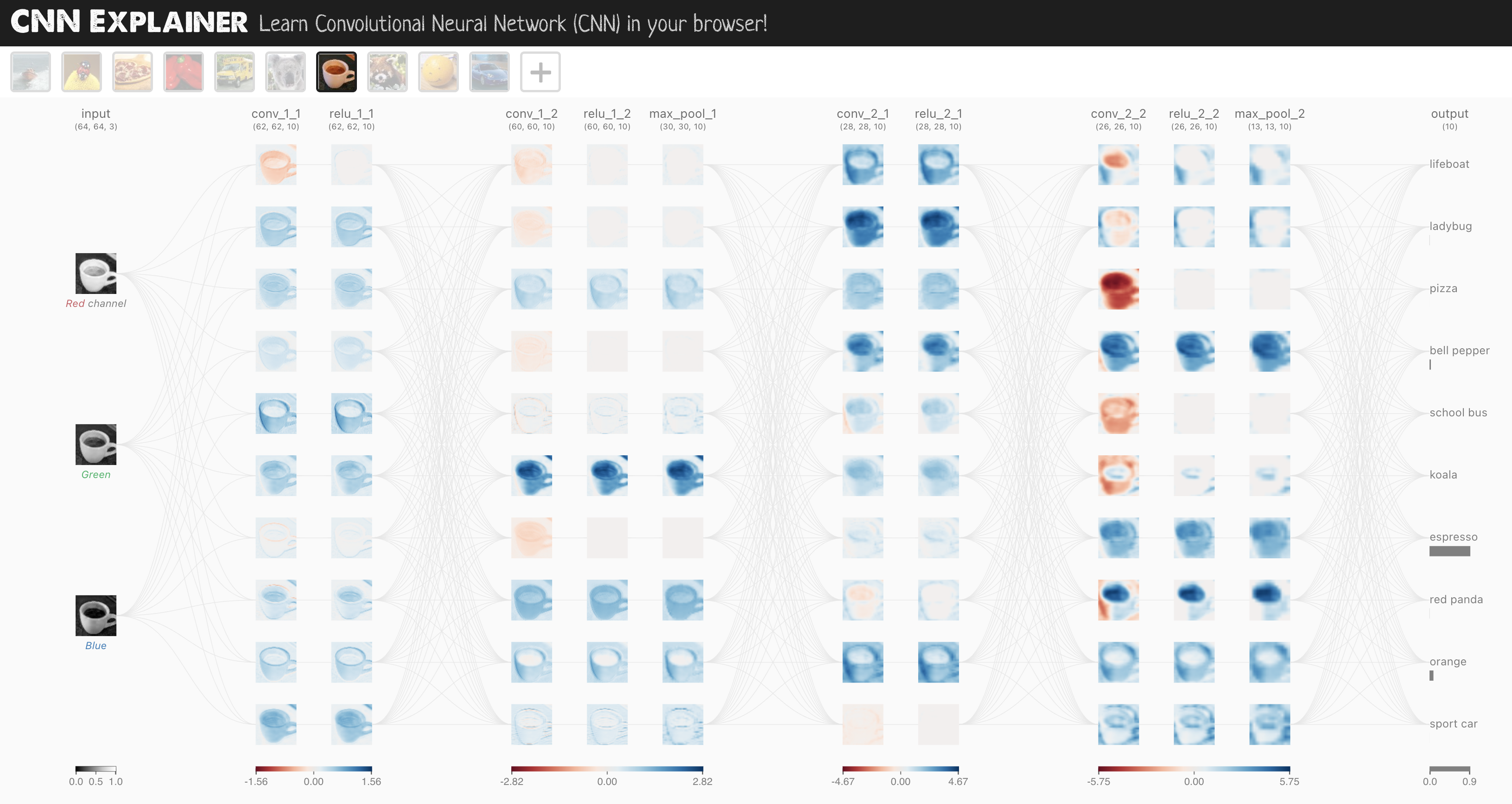
To do so, we’ll leverage the nn.Conv2d() and nn.MaxPool2d() layers from torch.nn.
# Create a convolutional neural network
class FashionMNISTModelV2(nn.Module):
    """
    Model architecture copying TinyVGG from:
    https://poloclub.github.io/cnn-explainer/
    """

    def __init__(self, input_shape: int, hidden_units: int, output_shape: int):
        super().__init__()
        self.block_1 = nn.Sequential(
            nn.Conv2d(
                in_channels=input_shape,
                out_channels=hidden_units,
                kernel_size=3,  # how big is the square that's going over the image?
                stride=1,  # default
                padding=1,
            ),  # options = "valid" (no padding) or "same" (output has same shape as input) or int for specific number
            nn.ReLU(),
            nn.Conv2d(
                in_channels=hidden_units,
                out_channels=hidden_units,
                kernel_size=3,
                stride=1,
                padding=1,
            ),
            nn.ReLU(),
            nn.MaxPool2d(
                kernel_size=2, stride=2
            ),  # default stride value is same as kernel_size
        )
        self.block_2 = nn.Sequential(
            nn.Conv2d(hidden_units, hidden_units, 3, padding=1),
            nn.ReLU(),
            nn.Conv2d(hidden_units, hidden_units, 3, padding=1),
            nn.ReLU(),
            nn.MaxPool2d(2),
        )
        self.classifier = nn.Sequential(
            nn.Flatten(),
            # Where did this in_features shape come from?
            # It's because each layer of our network compresses and changes the shape of our input data.
            nn.Linear(in_features=hidden_units * 7 * 7, out_features=output_shape),
        )

    def forward(self, x: torch.Tensor):
        x = self.block_1(x)
        # print(x.shape)
        x = self.block_2(x)
        # print(x.shape)
        x = self.classifier(x)
        # print(x.shape)
        return x


torch.manual_seed(42)
model_2 = FashionMNISTModelV2(
    input_shape=1, hidden_units=10, output_shape=len(class_names)
).to(device)
model_2
FashionMNISTModelV2(
  (block_1): Sequential(
    (0): Conv2d(1, 10, kernel_size=(3, 3), stride=(1, 1), padding=(1, 1))
    (1): ReLU()
    (2): Conv2d(10, 10, kernel_size=(3, 3), stride=(1, 1), padding=(1, 1))
    (3): ReLU()
    (4): MaxPool2d(kernel_size=2, stride=2, padding=0, dilation=1, ceil_mode=False)
  )
  (block_2): Sequential(
    (0): Conv2d(10, 10, kernel_size=(3, 3), stride=(1, 1), padding=(1, 1))
    (1): ReLU()
    (2): Conv2d(10, 10, kernel_size=(3, 3), stride=(1, 1), padding=(1, 1))
    (3): ReLU()
    (4): MaxPool2d(kernel_size=2, stride=2, padding=0, dilation=1, ceil_mode=False)
  )
  (classifier): Sequential(
    (0): Flatten(start_dim=1, end_dim=-1)
    (1): Linear(in_features=490, out_features=10, bias=True)
  )
)
This is our biggest model yet!
What we’ve done is a common practice in machine learning.
Find a model architecture somewhere and replicate it with code.
7.1 Stepping through nn.Conv2d()#
Ffirst step through the two new layers we’ve added:
nn.Conv2d(), also known as a convolutional layer.nn.MaxPool2d(), also known as a max pooling layer.
To test the layers out, let’s create some toy data just like the data used on CNN Explainer.
torch.manual_seed(42)

# Create sample batch of random numbers with same size as image batch
images = torch.randn(
    size=(32, 3, 64, 64)
)  # [batch_size, color_channels, height, width]
test_image = images[0]  # get a single image for testing

print(
    f"Image batch shape: {images.shape} -> [batch_size, color_channels, height, width]"
)
print(f"Single image shape: {test_image.shape} -> [color_channels, height, width]")
print(f"Single image pixel values:\n{test_image}")
Image batch shape: torch.Size([32, 3, 64, 64]) -> [batch_size, color_channels, height, width]
Single image shape: torch.Size([3, 64, 64]) -> [color_channels, height, width]
Single image pixel values:
tensor([[[ 1.9269,  1.4873,  0.9007,  ...,  1.8446, -1.1845,  1.3835],
         [ 1.4451,  0.8564,  2.2181,  ...,  0.3399,  0.7200,  0.4114],
         [ 1.9312,  1.0119, -1.4364,  ..., -0.5558,  0.7043,  0.7099],
         ...,
         [-0.5610, -0.4830,  0.4770,  ..., -0.2713, -0.9537, -0.6737],
         [ 0.3076, -0.1277,  0.0366,  ..., -2.0060,  0.2824, -0.8111],
         [-1.5486,  0.0485, -0.7712,  ..., -0.1403,  0.9416, -0.0118]],

        [[-0.5197,  1.8524,  1.8365,  ...,  0.8935, -1.5114, -0.8515],
         [ 2.0818,  1.0677, -1.4277,  ...,  1.6612, -2.6223, -0.4319],
         [-0.1010, -0.4388, -1.9775,  ...,  0.2106,  0.2536, -0.7318],
         ...,
         [ 0.2779,  0.7342, -0.3736,  ..., -0.4601,  0.1815,  0.1850],
         [ 0.7205, -0.2833,  0.0937,  ..., -0.1002, -2.3609,  2.2465],
         [-1.3242, -0.1973,  0.2920,  ...,  0.5409,  0.6940,  1.8563]],

        [[-0.7978,  1.0261,  1.1465,  ...,  1.2134,  0.9354, -0.0780],
         [-1.4647, -1.9571,  0.1017,  ..., -1.9986, -0.7409,  0.7011],
         [-1.3938,  0.8466, -1.7191,  ..., -1.1867,  0.1320,  0.3407],
         ...,
         [ 0.8206, -0.3745,  1.2499,  ..., -0.0676,  0.0385,  0.6335],
         [-0.5589, -0.3393,  0.2347,  ...,  2.1181,  2.4569,  1.3083],
         [-0.4092,  1.5199,  0.2401,  ..., -0.2558,  0.7870,  0.9924]]])
Let’s create an example nn.Conv2d() with various parameters:
in_channels(int) - Number of channels in the input image.out_channels(int) - Number of channels produced by the convolution.kernel_size(int or tuple) - Size of the convolving kernel/filter.stride(int or tuple, optional) - How big of a step the convolving kernel takes at a time. Default: 1.padding(int, tuple, str) - Padding added to all four sides of input. Default: 0.
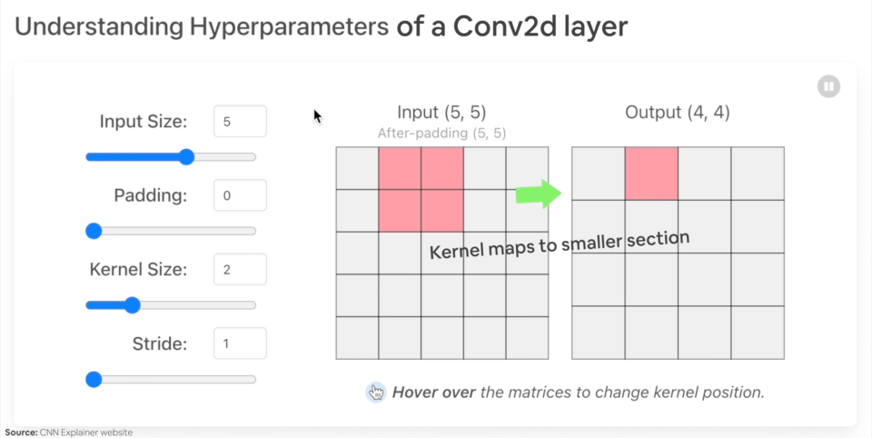
Example of what happens when you change the hyperparameters of a nn.Conv2d() layer.
torch.manual_seed(42)

# Create a convolutional layer with same dimensions as TinyVGG
# (try changing any of the parameters and see what happens)
conv_layer = nn.Conv2d(
    in_channels=3, out_channels=10, kernel_size=3, stride=1, padding=0
)  # also try using "valid" or "same" here

# Pass the data through the convolutional layer
conv_layer(
    test_image
)  # Note: If running PyTorch <1.11.0, this will error because of shape issues (nn.Conv.2d() expects a 4d tensor as input)
tensor([[[ 1.5396,  0.0516,  0.6454,  ..., -0.3673,  0.8711,  0.4256],
         [ 0.3662,  1.0114, -0.5997,  ...,  0.8983,  0.2809, -0.2741],
         [ 1.2664, -1.4054,  0.3727,  ..., -0.3409,  1.2191, -0.0463],
         ...,
         [-0.1541,  0.5132, -0.3624,  ..., -0.2360, -0.4609, -0.0035],
         [ 0.2981, -0.2432,  1.5012,  ..., -0.6289, -0.7283, -0.5767],
         [-0.0386, -0.0781, -0.0388,  ...,  0.2842,  0.4228, -0.1802]],

        [[-0.2840, -0.0319, -0.4455,  ..., -0.7956,  1.5599, -1.2449],
         [ 0.2753, -0.1262, -0.6541,  ..., -0.2211,  0.1999, -0.8856],
         [-0.5404, -1.5489,  0.0249,  ..., -0.5932, -1.0913, -0.3849],
         ...,
         [ 0.3870, -0.4064, -0.8236,  ...,  0.1734, -0.4330, -0.4951],
         [-0.1984, -0.6386,  1.0263,  ..., -0.9401, -0.0585, -0.7833],
         [-0.6306, -0.2052, -0.3694,  ..., -1.3248,  0.2456, -0.7134]],

        [[ 0.4414,  0.5100,  0.4846,  ..., -0.8484,  0.2638,  1.1258],
         [ 0.8117,  0.3191, -0.0157,  ...,  1.2686,  0.2319,  0.5003],
         [ 0.3212,  0.0485, -0.2581,  ...,  0.2258,  0.2587, -0.8804],
         ...,
         [-0.1144, -0.1869,  0.0160,  ..., -0.8346,  0.0974,  0.8421],
         [ 0.2941,  0.4417,  0.5866,  ..., -0.1224,  0.4814, -0.4799],
         [ 0.6059, -0.0415, -0.2028,  ...,  0.1170,  0.2521, -0.4372]],

        ...,

        [[-0.2560, -0.0477,  0.6380,  ...,  0.6436,  0.7553, -0.7055],
         [ 1.5595, -0.2209, -0.9486,  ..., -0.4876,  0.7754,  0.0750],
         [-0.0797,  0.2471,  1.1300,  ...,  0.1505,  0.2354,  0.9576],
         ...,
         [ 1.1065,  0.6839,  1.2183,  ...,  0.3015, -0.1910, -0.1902],
         [-0.3486, -0.7173, -0.3582,  ...,  0.4917,  0.7219,  0.1513],
         [ 0.0119,  0.1017,  0.7839,  ..., -0.3752, -0.8127, -0.1257]],

        [[ 0.3841,  1.1322,  0.1620,  ...,  0.7010,  0.0109,  0.6058],
         [ 0.1664,  0.1873,  1.5924,  ...,  0.3733,  0.9096, -0.5399],
         [ 0.4094, -0.0861, -0.7935,  ..., -0.1285, -0.9932, -0.3013],
         ...,
         [ 0.2688, -0.5630, -1.1902,  ...,  0.4493,  0.5404, -0.0103],
         [ 0.0535,  0.4411,  0.5313,  ...,  0.0148, -1.0056,  0.3759],
         [ 0.3031, -0.1590, -0.1316,  ..., -0.5384, -0.4271, -0.4876]],

        [[-1.1865, -0.7280, -1.2331,  ..., -0.9013, -0.0542, -1.5949],
         [-0.6345, -0.5920,  0.5326,  ..., -1.0395, -0.7963, -0.0647],
         [-0.1132,  0.5166,  0.2569,  ...,  0.5595, -1.6881,  0.9485],
         ...,
         [-0.0254, -0.2669,  0.1927,  ..., -0.2917,  0.1088, -0.4807],
         [-0.2609, -0.2328,  0.1404,  ..., -0.1325, -0.8436, -0.7524],
         [-1.1399, -0.1751, -0.8705,  ...,  0.1589,  0.3377,  0.3493]]],
       grad_fn=<SqueezeBackward1>)
Right now our single image test_image only has a shape of [color_channels, height, width] or [3, 64, 64].
We can fix this for a single image using test_image.unsqueeze(dim=0) to add an extra dimension for N. todo: what is N here - number of images? Maybe state the meaning explicitly
test_image.unsqueeze(dim=0).shape
torch.Size([1, 3, 64, 64])
# Pass test image with extra dimension through conv_layer
conv_layer(test_image.unsqueeze(dim=0)).shape
torch.Size([1, 10, 62, 62])
Notice what happens to the shape (the same as the first layer of TinyVGG on CNN Explainer).
Both the channel count and the pixel dimensions change.
What if we changed the values of conv_layer?
torch.manual_seed(42)
# Create a new conv_layer with different values (try setting these to whatever you like)
conv_layer_2 = nn.Conv2d(
    in_channels=3,  # same number of color channels as our input image
    out_channels=10,
    kernel_size=(5, 5),  # kernel is usually a square so a tuple also works
    stride=2,
    padding=0,
)

# Pass single image through new conv_layer_2 (this calls nn.Conv2d()'s forward() method on the input)
conv_layer_2(test_image.unsqueeze(dim=0)).shape
torch.Size([1, 10, 30, 30])
We get another shape change.
Now our image is of shape [1, 10, 30, 30] (it will be different if you use different values) or [batch_size=1, color_channels=10, height=30, width=30].
What’s happening?
Behind the scenes, nn.Conv2d() is compressing the information in the image by running operations on the input (our test image) against its internal parameters.
The goal here is similar to all of the other neural networks we’ve been building.
Data goes in and the layers try to update their internal parameters (patterns) to lower the loss function thanks to some help of the optimizer.
The only difference is how the different layers calculate their parameter updates or in PyTorch terms, the operation present in the layer forward() method.
If we check out our conv_layer_2.state_dict() we’ll find a similar weight and bias setup as we’ve seen before.
# Check out the conv_layer_2 internal parameters
print(conv_layer_2.state_dict())
OrderedDict({'weight': tensor([[[[ 0.0883,  0.0958, -0.0271,  0.1061, -0.0253],
          [ 0.0233, -0.0562,  0.0678,  0.1018, -0.0847],
          [ 0.1004,  0.0216,  0.0853,  0.0156,  0.0557],
          [-0.0163,  0.0890,  0.0171, -0.0539,  0.0294],
          [-0.0532, -0.0135, -0.0469,  0.0766, -0.0911]],

         [[-0.0532, -0.0326, -0.0694,  0.0109, -0.1140],
          [ 0.1043, -0.0981,  0.0891,  0.0192, -0.0375],
          [ 0.0714,  0.0180,  0.0933,  0.0126, -0.0364],
          [ 0.0310, -0.0313,  0.0486,  0.1031,  0.0667],
          [-0.0505,  0.0667,  0.0207,  0.0586, -0.0704]],

         [[-0.1143, -0.0446, -0.0886,  0.0947,  0.0333],
          [ 0.0478,  0.0365, -0.0020,  0.0904, -0.0820],
          [ 0.0073, -0.0788,  0.0356, -0.0398,  0.0354],
          [-0.0241,  0.0958, -0.0684, -0.0689, -0.0689],
          [ 0.1039,  0.0385,  0.1111, -0.0953, -0.1145]]],


        [[[-0.0903, -0.0777,  0.0468,  0.0413,  0.0959],
          [-0.0596, -0.0787,  0.0613, -0.0467,  0.0701],
          [-0.0274,  0.0661, -0.0897, -0.0583,  0.0352],
          [ 0.0244, -0.0294,  0.0688,  0.0785, -0.0837],
          [-0.0616,  0.1057, -0.0390, -0.0409, -0.1117]],

         [[-0.0661,  0.0288, -0.0152, -0.0838,  0.0027],
          [-0.0789, -0.0980, -0.0636, -0.1011, -0.0735],
          [ 0.1154,  0.0218,  0.0356, -0.1077, -0.0758],
          [-0.0384,  0.0181, -0.1016, -0.0498, -0.0691],
          [ 0.0003, -0.0430, -0.0080, -0.0782, -0.0793]],

         [[-0.0674, -0.0395, -0.0911,  0.0968, -0.0229],
          [ 0.0994,  0.0360, -0.0978,  0.0799, -0.0318],
          [-0.0443, -0.0958, -0.1148,  0.0330, -0.0252],
          [ 0.0450, -0.0948,  0.0857, -0.0848, -0.0199],
          [ 0.0241,  0.0596,  0.0932,  0.1052, -0.0916]]],


        [[[ 0.0291, -0.0497, -0.0127, -0.0864,  0.1052],
          [-0.0847,  0.0617,  0.0406,  0.0375, -0.0624],
          [ 0.1050,  0.0254,  0.0149, -0.1018,  0.0485],
          [-0.0173, -0.0529,  0.0992,  0.0257, -0.0639],
          [-0.0584, -0.0055,  0.0645, -0.0295, -0.0659]],

         [[-0.0395, -0.0863,  0.0412,  0.0894, -0.1087],
          [ 0.0268,  0.0597,  0.0209, -0.0411,  0.0603],
          [ 0.0607,  0.0432, -0.0203, -0.0306,  0.0124],
          [-0.0204, -0.0344,  0.0738,  0.0992, -0.0114],
          [-0.0259,  0.0017, -0.0069,  0.0278,  0.0324]],

         [[-0.1049, -0.0426,  0.0972,  0.0450, -0.0057],
          [-0.0696, -0.0706, -0.1034, -0.0376,  0.0390],
          [ 0.0736,  0.0533, -0.1021, -0.0694, -0.0182],
          [ 0.1117,  0.0167, -0.0299,  0.0478, -0.0440],
          [-0.0747,  0.0843, -0.0525, -0.0231, -0.1149]]],


        [[[ 0.0773,  0.0875,  0.0421, -0.0805, -0.1140],
          [-0.0938,  0.0861,  0.0554,  0.0972,  0.0605],
          [ 0.0292, -0.0011, -0.0878, -0.0989, -0.1080],
          [ 0.0473, -0.0567, -0.0232, -0.0665, -0.0210],
          [-0.0813, -0.0754,  0.0383, -0.0343,  0.0713]],

         [[-0.0370, -0.0847, -0.0204, -0.0560, -0.0353],
          [-0.1099,  0.0646, -0.0804,  0.0580,  0.0524],
          [ 0.0825, -0.0886,  0.0830, -0.0546,  0.0428],
          [ 0.1084, -0.0163, -0.0009, -0.0266, -0.0964],
          [ 0.0554, -0.1146,  0.0717,  0.0864,  0.1092]],

         [[-0.0272, -0.0949,  0.0260,  0.0638, -0.1149],
          [-0.0262, -0.0692, -0.0101, -0.0568, -0.0472],
          [-0.0367, -0.1097,  0.0947,  0.0968, -0.0181],
          [-0.0131, -0.0471, -0.1043, -0.1124,  0.0429],
          [-0.0634, -0.0742, -0.0090, -0.0385, -0.0374]]],


        [[[ 0.0037, -0.0245, -0.0398, -0.0553, -0.0940],
          [ 0.0968, -0.0462,  0.0306, -0.0401,  0.0094],
          [ 0.1077,  0.0532, -0.1001,  0.0458,  0.1096],
          [ 0.0304,  0.0774,  0.1138, -0.0177,  0.0240],
          [-0.0803, -0.0238,  0.0855,  0.0592, -0.0731]],

         [[-0.0926, -0.0789, -0.1140, -0.0891, -0.0286],
          [ 0.0779,  0.0193, -0.0878, -0.0926,  0.0574],
          [-0.0859, -0.0142,  0.0554, -0.0534, -0.0126],
          [-0.0101, -0.0273, -0.0585, -0.1029, -0.0933],
          [-0.0618,  0.1115, -0.0558, -0.0775,  0.0280]],

         [[ 0.0318,  0.0633,  0.0878,  0.0643, -0.1145],
          [ 0.0102,  0.0699, -0.0107, -0.0680,  0.1101],
          [-0.0432, -0.0657, -0.1041,  0.0052,  0.0512],
          [ 0.0256,  0.0228, -0.0876, -0.1078,  0.0020],
          [ 0.1053,  0.0666, -0.0672, -0.0150, -0.0851]]],


        [[[-0.0557,  0.0209,  0.0629,  0.0957, -0.1060],
          [ 0.0772, -0.0814,  0.0432,  0.0977,  0.0016],
          [ 0.1051, -0.0984, -0.0441,  0.0673, -0.0252],
          [-0.0236, -0.0481,  0.0796,  0.0566,  0.0370],
          [-0.0649, -0.0937,  0.0125,  0.0342, -0.0533]],

         [[-0.0323,  0.0780,  0.0092,  0.0052, -0.0284],
          [-0.1046, -0.1086, -0.0552, -0.0587,  0.0360],
          [-0.0336, -0.0452,  0.1101,  0.0402,  0.0823],
          [-0.0559, -0.0472,  0.0424, -0.0769, -0.0755],
          [-0.0056, -0.0422, -0.0866,  0.0685,  0.0929]],

         [[ 0.0187, -0.0201, -0.1070, -0.0421,  0.0294],
          [ 0.0544, -0.0146, -0.0457,  0.0643, -0.0920],
          [ 0.0730, -0.0448,  0.0018, -0.0228,  0.0140],
          [-0.0349,  0.0840, -0.0030,  0.0901,  0.1110],
          [-0.0563, -0.0842,  0.0926,  0.0905, -0.0882]]],


        [[[-0.0089, -0.1139, -0.0945,  0.0223,  0.0307],
          [ 0.0245, -0.0314,  0.1065,  0.0165, -0.0681],
          [-0.0065,  0.0277,  0.0404, -0.0816,  0.0433],
          [-0.0590, -0.0959, -0.0631,  0.1114,  0.0987],
          [ 0.1034,  0.0678,  0.0872, -0.0155, -0.0635]],

         [[ 0.0577, -0.0598, -0.0779, -0.0369,  0.0242],
          [ 0.0594, -0.0448, -0.0680,  0.0156, -0.0681],
          [-0.0752,  0.0602, -0.0194,  0.1055,  0.1123],
          [ 0.0345,  0.0397,  0.0266,  0.0018, -0.0084],
          [ 0.0016,  0.0431,  0.1074, -0.0299, -0.0488]],

         [[-0.0280, -0.0558,  0.0196,  0.0862,  0.0903],
          [ 0.0530, -0.0850, -0.0620, -0.0254, -0.0213],
          [ 0.0095, -0.1060,  0.0359, -0.0881, -0.0731],
          [-0.0960,  0.1006, -0.1093,  0.0871, -0.0039],
          [-0.0134,  0.0722, -0.0107,  0.0724,  0.0835]]],


        [[[-0.1003,  0.0444,  0.0218,  0.0248,  0.0169],
          [ 0.0316, -0.0555, -0.0148,  0.1097,  0.0776],
          [-0.0043, -0.1086,  0.0051, -0.0786,  0.0939],
          [-0.0701, -0.0083, -0.0256,  0.0205,  0.1087],
          [ 0.0110,  0.0669,  0.0896,  0.0932, -0.0399]],

         [[-0.0258,  0.0556, -0.0315,  0.0541, -0.0252],
          [-0.0783,  0.0470,  0.0177,  0.0515,  0.1147],
          [ 0.0788,  0.1095,  0.0062, -0.0993, -0.0810],
          [-0.0717, -0.1018, -0.0579, -0.1063, -0.1065],
          [-0.0690, -0.1138, -0.0709,  0.0440,  0.0963]],

         [[-0.0343, -0.0336,  0.0617, -0.0570, -0.0546],
          [ 0.0711, -0.1006,  0.0141,  0.1020,  0.0198],
          [ 0.0314, -0.0672, -0.0016,  0.0063,  0.0283],
          [ 0.0449,  0.1003, -0.0881,  0.0035, -0.0577],
          [-0.0913, -0.0092, -0.1016,  0.0806,  0.0134]]],


        [[[-0.0622,  0.0603, -0.1093, -0.0447, -0.0225],
          [-0.0981, -0.0734, -0.0188,  0.0876,  0.1115],
          [ 0.0735, -0.0689, -0.0755,  0.1008,  0.0408],
          [ 0.0031,  0.0156, -0.0928, -0.0386,  0.1112],
          [-0.0285, -0.0058, -0.0959, -0.0646, -0.0024]],

         [[-0.0717, -0.0143,  0.0470, -0.1130,  0.0343],
          [-0.0763, -0.0564,  0.0443,  0.0918, -0.0316],
          [-0.0474, -0.1044, -0.0595, -0.1011, -0.0264],
          [ 0.0236, -0.1082,  0.1008,  0.0724, -0.1130],
          [-0.0552,  0.0377, -0.0237, -0.0126, -0.0521]],

         [[ 0.0927, -0.0645,  0.0958,  0.0075,  0.0232],
          [ 0.0901, -0.0190, -0.0657, -0.0187,  0.0937],
          [-0.0857,  0.0262, -0.1135,  0.0605,  0.0427],
          [ 0.0049,  0.0496,  0.0001,  0.0639, -0.0914],
          [-0.0170,  0.0512,  0.1150,  0.0588, -0.0840]]],


        [[[ 0.0888, -0.0257, -0.0247, -0.1050, -0.0182],
          [ 0.0817,  0.0161, -0.0673,  0.0355, -0.0370],
          [ 0.1054, -0.1002, -0.0365, -0.1115, -0.0455],
          [ 0.0364,  0.1112,  0.0194,  0.1132,  0.0226],
          [ 0.0667,  0.0926,  0.0965, -0.0646,  0.1062]],

         [[ 0.0699, -0.0540, -0.0551, -0.0969,  0.0290],
          [-0.0936,  0.0488,  0.0365, -0.1003,  0.0315],
          [-0.0094,  0.0527,  0.0663, -0.1148,  0.1059],
          [ 0.0968,  0.0459, -0.1055, -0.0412, -0.0335],
          [-0.0297,  0.0651,  0.0420,  0.0915, -0.0432]],

         [[ 0.0389,  0.0411, -0.0961, -0.1120, -0.0599],
          [ 0.0790, -0.1087, -0.1005,  0.0647,  0.0623],
          [ 0.0950, -0.0872, -0.0845,  0.0592,  0.1004],
          [ 0.0691,  0.0181,  0.0381,  0.1096, -0.0745],
          [-0.0524,  0.0808, -0.0790, -0.0637,  0.0843]]]]), 'bias': tensor([ 0.0364,  0.0373, -0.0489, -0.0016,  0.1057, -0.0693,  0.0009,  0.0549,
        -0.0797,  0.1121])})
As a result, we get a bunch of random numbers for a weight and bias tensor.
The shapes of these are manipulated by the inputs we passed to nn.Conv2d() when we set it up.
# Get shapes of weight and bias tensors within conv_layer_2
print(
    f"conv_layer_2 weight shape: \n{conv_layer_2.weight.shape} -> [out_channels=10, in_channels=3, kernel_size=5, kernel_size=5]"
)
print(f"\nconv_layer_2 bias shape: \n{conv_layer_2.bias.shape} -> [out_channels=10]")
conv_layer_2 weight shape:
torch.Size([10, 3, 5, 5]) -> [out_channels=10, in_channels=3, kernel_size=5, kernel_size=5]

conv_layer_2 bias shape:
torch.Size([10]) -> [out_channels=10]
How should we set the parameters of nn.Conv2d()?
Similar to many other things in machine learning, the values of these aren’t set in stone (and remember, because these values are the ones we can set ourselves, they’re referred to as “hyperparameters”).
The best way to find out is to try out different values and see how they affect your model’s performance.
Or even better, find a working example on a problem similar to yours (like we’ve done with TinyVGG) and copy it.
We’re working with a different type of layer here to what we’ve seen before.
But the premise remains the same: start with random numbers and update them to better represent the data.
7.2 Stepping through nn.MaxPool2d()#
Now let’s check out what happens when we move data through nn.MaxPool2d().
# Print out original image shape without and with unsqueezed dimension
print(f"Test image original shape: {test_image.shape}")
print(f"Test image with unsqueezed dimension: {test_image.unsqueeze(dim=0).shape}")

# Create a sample nn.MaxPoo2d() layer
max_pool_layer = nn.MaxPool2d(kernel_size=2)

# Pass data through just the conv_layer
test_image_through_conv = conv_layer(test_image.unsqueeze(dim=0))
print(f"Shape after going through conv_layer(): {test_image_through_conv.shape}")

# Pass data through the max pool layer
test_image_through_conv_and_max_pool = max_pool_layer(test_image_through_conv)
print(
    f"Shape after going through conv_layer() and max_pool_layer(): {test_image_through_conv_and_max_pool.shape}"
)
Test image original shape: torch.Size([3, 64, 64])
Test image with unsqueezed dimension: torch.Size([1, 3, 64, 64])
Shape after going through conv_layer(): torch.Size([1, 10, 62, 62])
Shape after going through conv_layer() and max_pool_layer(): torch.Size([1, 10, 31, 31])
Notice the change in the shapes of what’s happening in and out of a nn.MaxPool2d() layer.
The kernel_size of the nn.MaxPool2d() layer will affect the size of the output shape.
In our case, the shape halves from a 62x62 image to 31x31 image.
Let’s see this work with a smaller tensor.
torch.manual_seed(42)
# Create a random tensor with a similar number of dimensions to our images
random_tensor = torch.randn(size=(1, 1, 2, 2))
print(f"Random tensor:\n{random_tensor}")
print(f"Random tensor shape: {random_tensor.shape}")

# Create a max pool layer
max_pool_layer = nn.MaxPool2d(
    kernel_size=2
)  # see what happens when you change the kernel_size value

# Pass the random tensor through the max pool layer
max_pool_tensor = max_pool_layer(random_tensor)
print(
    f"\nMax pool tensor:\n{max_pool_tensor} <- this is the maximum value from random_tensor"
)
print(f"Max pool tensor shape: {max_pool_tensor.shape}")
Random tensor:
tensor([[[[0.3367, 0.1288],
          [0.2345, 0.2303]]]])
Random tensor shape: torch.Size([1, 1, 2, 2])

Max pool tensor:
tensor([[[[0.3367]]]]) <- this is the maximum value from random_tensor
Max pool tensor shape: torch.Size([1, 1, 1, 1])
The final two dimensions between random_tensor and max_pool_tensor, they go from [2, 2] to [1, 1].
In essence, they get halved.
And the change would be different for different values of kernel_size for nn.MaxPool2d().
Also the value leftover in max_pool_tensor is the maximum value from random_tensor.
What’s happening here?
This is another important piece of the puzzle of neural networks.
Essentially, every layer in a neural network is trying to compress data from higher dimensional space to lower dimensional space.
In other words, take a lot of numbers (raw data) and learn patterns in those numbers, patterns that are predictive whilst also being smaller in size than the original values.
From an artificial intelligence perspective, you could consider the whole goal of a neural network is to compress information.
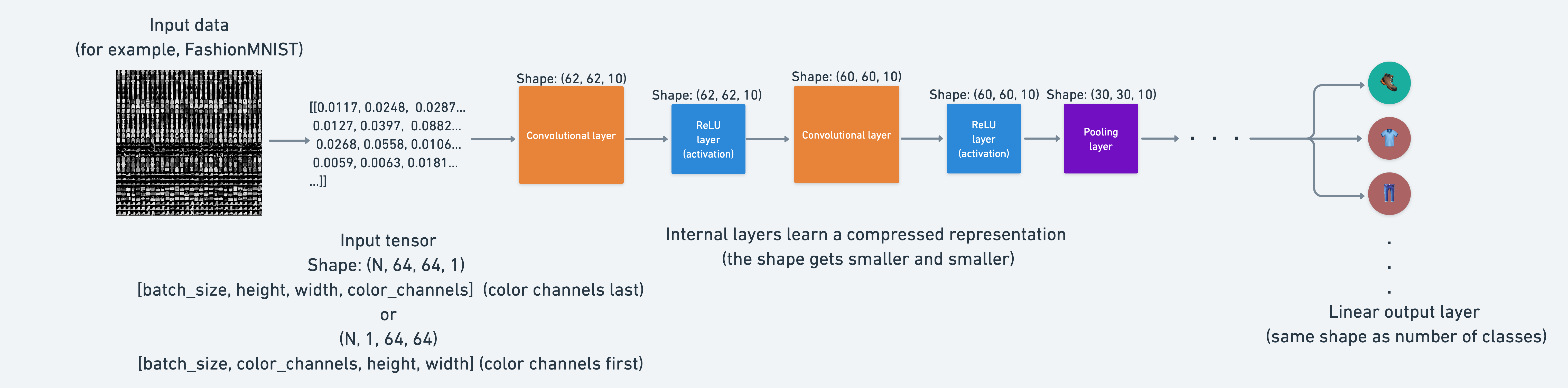
This means, that from the point of view of a neural network, intelligence is compression.
This is the idea of the use of a nn.MaxPool2d() layer: take the maximum value from a portion of a tensor and disregard the rest.
In essence, lowering the dimensionality of a tensor whilst still retaining a (hopefully) significant portion of the information.
It is the same story for a nn.Conv2d() layer.
Except instead of just taking the maximum, the nn.Conv2d() performs a convolutional operation on the data (see this in action on the CNN Explainer webpage).
7.3 Setup a loss function and optimizer for model_2#
We’ve gone through the CNN layers in enough detail.
But remember, if something still isn’t clear, try starting small.
Pick a single layer of a model, pass some data through it and see what happens.
Time to get training.
Let’s setup a loss function and an optimizer.
We’ll use the functions as before, nn.CrossEntropyLoss() as the loss function (since we’re working with multi-class classification data).
And torch.optim.SGD() as the optimizer to optimize model_2.parameters() with a learning rate of 0.1.
# Setup loss and optimizer
loss_fn = nn.CrossEntropyLoss()
optimizer = torch.optim.SGD(params=model_2.parameters(), lr=0.1)
7.4 Training and testing model_2 using our training and test functions#
Loss and optimizer ready!
Time to train and test.
We’ll use our train_step() and test_step() functions we created before.
We’ll also measure the time to compare it to our other models.
torch.manual_seed(42)

# Measure time
from timeit import default_timer as timer

train_time_start_model_2 = timer()

# Train and test model
epochs = 3
for epoch in tqdm(range(epochs)):
    print(f"Epoch: {epoch}\n---------")
    train_step(
        data_loader=train_dataloader,
        model=model_2,
        loss_fn=loss_fn,
        optimizer=optimizer,
        accuracy_fn=accuracy_fn,
        device=device,
    )
    test_step(
        data_loader=test_dataloader,
        model=model_2,
        loss_fn=loss_fn,
        accuracy_fn=accuracy_fn,
        device=device,
    )

train_time_end_model_2 = timer()
total_train_time_model_2 = print_train_time(
    start=train_time_start_model_2, end=train_time_end_model_2, device=device
)
Epoch: 0
---------
Train loss: 0.59135 | Train accuracy: 78.47%
Test loss: 0.39805 | Test accuracy: 85.60%

Epoch: 1
---------
Train loss: 0.36091 | Train accuracy: 86.96%
Test loss: 0.35226 | Test accuracy: 87.21%

Epoch: 2
---------
Train loss: 0.32338 | Train accuracy: 88.29%
Test loss: 0.33501 | Test accuracy: 87.96%

Train time on cuda: 37.497 seconds
Looks like the convolutional and max pooling layers helped improve performance a little.
Let’s evaluate model_2’s results with our eval_model() function.
# Get model_2 results
model_2_results = eval_model(
    model=model_2, data_loader=test_dataloader, loss_fn=loss_fn, accuracy_fn=accuracy_fn
)
model_2_results
{'model_name': 'FashionMNISTModelV2',
 'model_loss': 0.3350149095058441,
 'model_acc': 87.95926517571885}
8. Compare model results and training time#
We’ve trained three different models.
model_0- our baseline model with twonn.Linear()layers.model_1- the same setup as our baseline model except withnn.ReLU()layers in between thenn.Linear()layers.model_2- our first CNN model that mimics the TinyVGG architecture
This is a regular practice in machine learning.
Building multiple models and performing multiple training experiments to see which performs best.
Now combine our model results dictionaries into a DataFrame and find out.
import pandas as pd

compare_results = pd.DataFrame([model_0_results, model_1_results, model_2_results])
compare_results
| model_name | model_loss | model_acc | |
|---|---|---|---|
| 0 | FashionMNISTModelV0 | 0.476639 | 83.426518 |
| 1 | FashionMNISTModelV1 | 0.685001 | 75.019968 |
| 2 | FashionMNISTModelV2 | 0.335015 | 87.959265 |
We can add the training time values too.
# Add training times to results comparison
compare_results["training_time"] = [
    total_train_time_model_0,
    total_train_time_model_1,
    total_train_time_model_2,
]
compare_results
| model_name | model_loss | model_acc | training_time | |
|---|---|---|---|---|
| 0 | FashionMNISTModelV0 | 0.476639 | 83.426518 | 28.764266 |
| 1 | FashionMNISTModelV1 | 0.685001 | 75.019968 | 30.877928 |
| 2 | FashionMNISTModelV2 | 0.335015 | 87.959265 | 37.497049 |
It looks like our CNN (FashionMNISTModelV2) model performed the best (lowest loss, highest accuracy) but had the longest training time.
And our baseline model (FashionMNISTModelV0) performed better than model_1 (FashionMNISTModelV1).
Performance-speed tradeoff#
Something to be aware of in machine learning is the performance-speed tradeoff.
Generally, you get better performance out of a larger, more complex model (like we did with model_2).
However, this performance increase often comes at a sacrifice of training speed and inference speed.
Note: The training times you get will be very dependent on the hardware you use.
Generally, the more CPU cores you have, the faster your models will train on CPU. And similar for GPUs.
# Visualize our model results
compare_results.set_index("model_name")["model_acc"].plot(kind="barh")
plt.xlabel("accuracy (%)")
plt.ylabel("model");
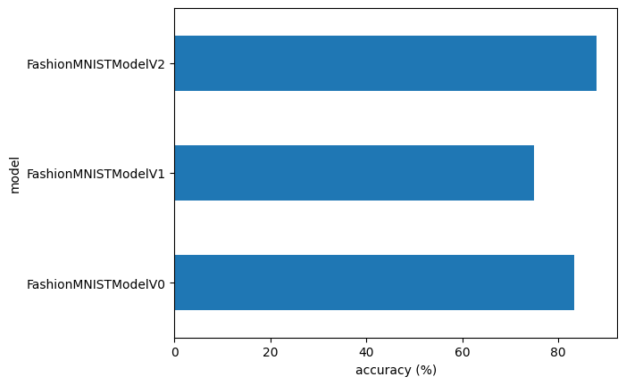
9. Make and evaluate random predictions with best model#
We’ve compared our models to each other, let’s further evaluate our best performing model, model_2.
To do so, let’s create a function make_predictions() where we can pass the model and some data for it to predict on.
def make_predictions(model: torch.nn.Module, data: list, device: torch.device = device):
    pred_probs = []
    model.eval()
    with torch.inference_mode():
        for sample in data:
            # Prepare sample
            sample = torch.unsqueeze(sample, dim=0).to(
                device
            )  # Add an extra dimension and send sample to device

            # Forward pass (model outputs raw logit)
            pred_logit = model(sample)

            # Get prediction probability (logit -> prediction probability)
            pred_prob = torch.softmax(
                pred_logit.squeeze(), dim=0
            )  # note: perform softmax on the "logits" dimension, not "batch" dimension (in this case we have a batch size of 1, so can perform on dim=0)

            # Get pred_prob off GPU for further calculations
            pred_probs.append(pred_prob.cpu())

    # Stack the pred_probs to turn list into a tensor
    return torch.stack(pred_probs)
import random

random.seed(42)
test_samples = []
test_labels = []
for sample, label in random.sample(list(test_data), k=9):
    test_samples.append(sample)
    test_labels.append(label)

# View the first test sample shape and label
print(
    f"Test sample image shape: {test_samples[0].shape}\nTest sample label: {test_labels[0]} ({class_names[test_labels[0]]})"
)
Test sample image shape: torch.Size([1, 28, 28])
Test sample label: 5 (Sandal)
And now we can use our make_predictions() function to predict on test_samples.
# Make predictions on test samples with model 2
pred_probs = make_predictions(model=model_2, data=test_samples)

# View first two prediction probabilities list
pred_probs[:2]
tensor([[5.0434e-08, 3.4208e-09, 5.9504e-08, 1.3610e-08, 1.3439e-08, 9.9993e-01,
         2.3305e-07, 4.8576e-06, 1.7421e-05, 5.0785e-05],
        [1.0077e-01, 6.9387e-01, 3.7280e-04, 1.1955e-01, 3.4762e-02, 5.4889e-05,
         4.9340e-02, 6.2916e-04, 5.1972e-04, 1.3332e-04]])
We can go from prediction probabilities to prediction labels by taking the torch.argmax() of the output of the torch.softmax() activation function.
# Turn the prediction probabilities into prediction labels by taking the argmax()
pred_classes = pred_probs.argmax(dim=1)
pred_classes
tensor([5, 1, 7, 4, 3, 0, 4, 7, 1])
# Are our predictions in the same form as our test labels?
test_labels, pred_classes
([5, 1, 7, 4, 3, 0, 4, 7, 1], tensor([5, 1, 7, 4, 3, 0, 4, 7, 1]))
Now our predicted classes are in the same format as our test labels, we can compare.
Since we’re dealing with image data, let’s stay true to the data explorer’s motto.
“Visualize, visualize, visualize!”
# Plot predictions
plt.figure(figsize=(9, 9))
nrows = 3
ncols = 3
for i, sample in enumerate(test_samples):
    # Create a subplot
    plt.subplot(nrows, ncols, i + 1)

    # Plot the target image
    plt.imshow(sample.squeeze(), cmap="gray")

    # Find the prediction label (in text form, e.g. "Sandal")
    pred_label = class_names[pred_classes[i]]

    # Get the truth label (in text form, e.g. "T-shirt")
    truth_label = class_names[test_labels[i]]

    # Create the title text of the plot
    title_text = f"Pred: {pred_label} | Truth: {truth_label}"

    # Check for equality and change title colour accordingly
    if pred_label == truth_label:
        plt.title(title_text, fontsize=10, c="g")  # green text if correct
    else:
        plt.title(title_text, fontsize=10, c="r")  # red text if wrong
    plt.axis(False)
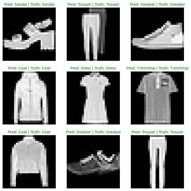
10. Making a confusion matrix for further prediction evaluation#
There are many different evaluation metrics we can use for classification problems.
One of the most visual is a confusion matrix.
A confusion matrix shows you where your classification model got confused between predictions and true labels.
To make a confusion matrix, we’ll go through three steps:
Make predictions with our trained model,
model_2(a confusion matrix compares predictions to true labels).Make a confusion matrix using
torchmetrics.ConfusionMatrix.Plot the confusion matrix using
mlxtend.plotting.plot_confusion_matrix().
Let’s start by making predictions with our trained model.
# Import tqdm for progress bar
from tqdm.auto import tqdm

# 1. Make predictions with trained model
y_preds = []
model_2.eval()
with torch.inference_mode():
    for X, y in tqdm(test_dataloader, desc="Making predictions"):
        # Send data and targets to target device
        X, y = X.to(device), y.to(device)
        # Do the forward pass
        y_logit = model_2(X)
        # Turn predictions from logits -> prediction probabilities -> predictions labels
        y_pred = torch.softmax(
            y_logit, dim=1
        ).argmax(
            dim=1
        )  # note: perform softmax on the "logits" dimension, not "batch" dimension (in this case we have a batch size of 32, so can perform on dim=1)
        # Put predictions on CPU for evaluation
        y_preds.append(y_pred.cpu())
# Concatenate list of predictions into a tensor
y_pred_tensor = torch.cat(y_preds)
Now we’ve got predictions, let’s go through steps 2 & 3:
Make a confusion matrix using
torchmetrics.ConfusionMatrix.Plot the confusion matrix using
mlxtend.plotting.plot_confusion_matrix().
First we’ll need to make sure we’ve got torchmetrics and mlxtend installed (these two libraries will help us make and visualize a confusion matrix).
# See if torchmetrics exists, if not, install it
try:
    import torchmetrics, mlxtend

    print(f"mlxtend version: {mlxtend.__version__}")
    assert int(mlxtend.__version__.split(".")[1]) >= 19, (
        "mlxtend version should be 0.19.0 or higher"
    )
except:
    !pip install -q -U numpy torchmetrics mlxtend
    import torchmetrics, mlxtend

    print(f"mlxtend version: {mlxtend.__version__}")
---------------------------------------------------------------------------
ImportError                               Traceback (most recent call last)
/tmp/ipykernel_3204/501281729.py in <cell line: 0>()
      2 try:
----> 3     import torchmetrics, mlxtend
      4

/usr/local/lib/python3.12/dist-packages/torchmetrics/__init__.py in <module>
     30 if package_available("scipy"):
---> 31     import scipy.signal
     32

/usr/local/lib/python3.12/dist-packages/scipy/signal/__init__.py in <module>
    300
--> 301 from ._support_alternative_backends import *
    302 from . import _support_alternative_backends

/usr/local/lib/python3.12/dist-packages/scipy/signal/_support_alternative_backends.py in <module>
      1 import functools
----> 2 from scipy._lib._array_api import (
      3     is_cupy, is_jax, scipy_namespace_for, SCIPY_ARRAY_API

/usr/local/lib/python3.12/dist-packages/scipy/_lib/_array_api.py in <module>
     24 from scipy._lib import array_api_compat
---> 25 from scipy._lib.array_api_compat import (
     26     is_array_api_obj,

/usr/local/lib/python3.12/dist-packages/scipy/_lib/array_api_compat/numpy/__init__.py in <module>
      3
----> 4 from numpy import *  # noqa: F403  # pyright: ignore[reportWildcardImportFromLibrary]
      5

/usr/local/lib/python3.12/dist-packages/numpy/__init__.py in __getattr__(attr)
    366         ptp,
--> 367         put,
    368         putmask,

/usr/local/lib/python3.12/dist-packages/numpy/char/__init__.py in <module>
----> 1 from numpy._core.defchararray import *
      2 from numpy._core.defchararray import __all__, __doc__

/usr/local/lib/python3.12/dist-packages/numpy/_core/defchararray.py in <module>
     22 from numpy._core.multiarray import compare_chararrays
---> 23 from numpy._core.strings import (
     24     _join as join,

/usr/local/lib/python3.12/dist-packages/numpy/_core/strings.py in <module>
     21 from numpy._core.overrides import array_function_dispatch, set_module
---> 22 from numpy._core.umath import (
     23     _center,

ImportError: cannot import name '_center' from 'numpy._core.umath' (/usr/local/lib/python3.12/dist-packages/numpy/_core/umath.py)

During handling of the above exception, another exception occurred:

ImportError                               Traceback (most recent call last)
/tmp/ipykernel_3204/501281729.py in <cell line: 0>()
      9 except:
     10     get_ipython().system('pip install -q -U numpy torchmetrics mlxtend')
---> 11     import torchmetrics, mlxtend
     12
     13     print(f"mlxtend version: {mlxtend.__version__}")

/usr/local/lib/python3.12/dist-packages/torchmetrics/__init__.py in <module>
     29
     30 if package_available("scipy"):
---> 31     import scipy.signal
     32
     33     # back compatibility patch due to SMRMpy using scipy.signal.hamming

/usr/local/lib/python3.12/dist-packages/scipy/signal/__init__.py in <module>
    299 # mypy: ignore-errors
    300
--> 301 from ._support_alternative_backends import *
    302 from . import _support_alternative_backends
    303 __all__ = _support_alternative_backends.__all__

/usr/local/lib/python3.12/dist-packages/scipy/signal/_support_alternative_backends.py in <module>
      1 import functools
----> 2 from scipy._lib._array_api import (
      3     is_cupy, is_jax, scipy_namespace_for, SCIPY_ARRAY_API
      4 )
      5

/usr/local/lib/python3.12/dist-packages/scipy/_lib/_array_api.py in <module>
     23
     24 from scipy._lib import array_api_compat
---> 25 from scipy._lib.array_api_compat import (
     26     is_array_api_obj,
     27     is_lazy_array,

/usr/local/lib/python3.12/dist-packages/scipy/_lib/array_api_compat/numpy/__init__.py in <module>
      2 from typing import Final
      3
----> 4 from numpy import *  # noqa: F403  # pyright: ignore[reportWildcardImportFromLibrary]
      5
      6 # from numpy import * doesn't overwrite these builtin names

/usr/local/lib/python3.12/dist-packages/numpy/__init__.py in __getattr__(attr)
    365         promote_types,
    366         ptp,
--> 367         put,
    368         putmask,
    369         rad2deg,

/usr/local/lib/python3.12/dist-packages/numpy/char/__init__.py in <module>
----> 1 from numpy._core.defchararray import *
      2 from numpy._core.defchararray import __all__, __doc__

/usr/local/lib/python3.12/dist-packages/numpy/_core/defchararray.py in <module>
     21 from numpy._core import overrides
     22 from numpy._core.multiarray import compare_chararrays
---> 23 from numpy._core.strings import (
     24     _join as join,
     25     _rsplit as rsplit,

/usr/local/lib/python3.12/dist-packages/numpy/_core/strings.py in <module>
     20 from numpy._core.multiarray import _vec_string
     21 from numpy._core.overrides import array_function_dispatch, set_module
---> 22 from numpy._core.umath import (
     23     _center,
     24     _expandtabs,

ImportError: cannot import name '_center' from 'numpy._core.umath' (/usr/local/lib/python3.12/dist-packages/numpy/_core/umath.py)

---------------------------------------------------------------------------
NOTE: If your import is failing due to a missing package, you can
manually install dependencies using either !pip or !apt.

To view examples of installing some common dependencies, click the
"Open Examples" button below.
---------------------------------------------------------------------------
Now that we have torchmetrics and mlxtend installed, let’s make a confusion matrix!
First we’ll create a torchmetrics.ConfusionMatrix instance telling it how many classes we’re dealing with by setting num_classes=len(class_names).
Then we’ll create a confusion matrix (in tensor format) by passing our instance our model’s predictions (preds=y_pred_tensor) and targets (target=test_data.targets).
Finally we can plot our confusion matrix using the plot_confusion_matrix() function from mlxtend.plotting.
from torchmetrics import ConfusionMatrix
from mlxtend.plotting import plot_confusion_matrix

# 2. Setup confusion matrix instance and compare predictions to targets
confmat = ConfusionMatrix(num_classes=len(class_names), task="multiclass")
confmat_tensor = confmat(preds=y_pred_tensor, target=test_data.targets)

# 3. Plot the confusion matrix
fig, ax = plot_confusion_matrix(
    conf_mat=confmat_tensor.numpy(),  # matplotlib likes working with NumPy
    class_names=class_names,  # turn the row and column labels into class names
    figsize=(10, 7),
)
---------------------------------------------------------------------------
ImportError                               Traceback (most recent call last)
/tmp/ipykernel_3204/252256104.py in <cell line: 0>()
----> 1 from torchmetrics import ConfusionMatrix
      2 from mlxtend.plotting import plot_confusion_matrix
      3
      4 # 2. Setup confusion matrix instance and compare predictions to targets
      5 confmat = ConfusionMatrix(num_classes=len(class_names), task="multiclass")

/usr/local/lib/python3.12/dist-packages/torchmetrics/__init__.py in <module>
     29
     30 if package_available("scipy"):
---> 31     import scipy.signal
     32
     33     # back compatibility patch due to SMRMpy using scipy.signal.hamming

/usr/local/lib/python3.12/dist-packages/scipy/signal/__init__.py in <module>
    299 # mypy: ignore-errors
    300
--> 301 from ._support_alternative_backends import *
    302 from . import _support_alternative_backends
    303 __all__ = _support_alternative_backends.__all__

/usr/local/lib/python3.12/dist-packages/scipy/signal/_support_alternative_backends.py in <module>
      1 import functools
----> 2 from scipy._lib._array_api import (
      3     is_cupy, is_jax, scipy_namespace_for, SCIPY_ARRAY_API
      4 )
      5

/usr/local/lib/python3.12/dist-packages/scipy/_lib/_array_api.py in <module>
     23
     24 from scipy._lib import array_api_compat
---> 25 from scipy._lib.array_api_compat import (
     26     is_array_api_obj,
     27     is_lazy_array,

/usr/local/lib/python3.12/dist-packages/scipy/_lib/array_api_compat/numpy/__init__.py in <module>
      2 from typing import Final
      3
----> 4 from numpy import *  # noqa: F403  # pyright: ignore[reportWildcardImportFromLibrary]
      5
      6 # from numpy import * doesn't overwrite these builtin names

/usr/local/lib/python3.12/dist-packages/numpy/__init__.py in __getattr__(attr)
    365         promote_types,
    366         ptp,
--> 367         put,
    368         putmask,
    369         rad2deg,

/usr/local/lib/python3.12/dist-packages/numpy/char/__init__.py in <module>
----> 1 from numpy._core.defchararray import *
      2 from numpy._core.defchararray import __all__, __doc__

/usr/local/lib/python3.12/dist-packages/numpy/_core/defchararray.py in <module>
     21 from numpy._core import overrides
     22 from numpy._core.multiarray import compare_chararrays
---> 23 from numpy._core.strings import (
     24     _join as join,
     25     _rsplit as rsplit,

/usr/local/lib/python3.12/dist-packages/numpy/_core/strings.py in <module>
     20 from numpy._core.multiarray import _vec_string
     21 from numpy._core.overrides import array_function_dispatch, set_module
---> 22 from numpy._core.umath import (
     23     _center,
     24     _expandtabs,

ImportError: cannot import name '_center' from 'numpy._core.umath' (/usr/local/lib/python3.12/dist-packages/numpy/_core/umath.py)

---------------------------------------------------------------------------
NOTE: If your import is failing due to a missing package, you can
manually install dependencies using either !pip or !apt.

To view examples of installing some common dependencies, click the
"Open Examples" button below.
---------------------------------------------------------------------------
We can see our model does fairly well since most of the dark squares run down the diagonal from top left to bottom right (an ideal model would have values only in these squares and 0 everywhere else).
The model gets most “confused” on classes that look similar, for example predicting “Pullover” for images actually labelled “Shirt”, and predicting “Shirt” for images actually labelled “T-shirt/top”.
This kind of information is often more useful than a single accuracy number, because it tells us where the model is getting things wrong, and hints at why. It’s understandable that the model sometimes predicts “Shirt” for images labelled “T-shirt/top”.
We can use this to dig further into our models and data and see how things could be improved.
11. Save and load best performing model#
Let’s finish this section off by saving and loading in our best performing model.
we can save and load a PyTorch model using a combination of:
torch.save- a function to save a whole PyTorch model or a model’sstate_dict().torch.load- a function to load in a saved PyTorch object.torch.nn.Module.load_state_dict()- a function to load a savedstate_dict()into an existing model instance.
You can see more of these three in the PyTorch saving and loading models documentation.
For now, let’s save our model_2’s state_dict() then load it back in and evaluate it to make sure the save and load went correctly.
from pathlib import Path

# Create models directory (if it doesn't already exist), see: https://docs.python.org/3/library/pathlib.html#pathlib.Path.mkdir
MODEL_PATH = Path("models")
MODEL_PATH.mkdir(
    parents=True,  # create parent directories if needed
    exist_ok=True,  # if models directory already exists, don't error
)

# Create model save path
MODEL_NAME = "03_pytorch_computer_vision_model_2.pth"
MODEL_SAVE_PATH = MODEL_PATH / MODEL_NAME

# Save the model state dict
print(f"Saving model to: {MODEL_SAVE_PATH}")
torch.save(
    obj=model_2.state_dict(),  # only saving the state_dict() only saves the learned parameters
    f=MODEL_SAVE_PATH,
)
Saving model to: models/03_pytorch_computer_vision_model_2.pth
Now we’ve got a saved model state_dict() we can load it back in using a combination of load_state_dict() and torch.load().
Since we’re using load_state_dict(), we’ll need to create a new instance of FashionMNISTModelV2() with the same input parameters as our saved model state_dict().
# Create a new instance of FashionMNISTModelV2 (the same class as our saved state_dict())
# Note: loading model will error if the shapes here aren't the same as the saved version
loaded_model_2 = FashionMNISTModelV2(
    input_shape=1,
    hidden_units=10,  # try changing this to 128 and seeing what happens
    output_shape=10,
)

# Load in the saved state_dict()
loaded_model_2.load_state_dict(torch.load(f=MODEL_SAVE_PATH))

# Send model to GPU
loaded_model_2 = loaded_model_2.to(device)
And now we’ve got a loaded model we can evaluate it with eval_model() to make sure its parameters work similarly to model_2 prior to saving.
# Evaluate loaded model
torch.manual_seed(42)

loaded_model_2_results = eval_model(
    model=loaded_model_2,
    data_loader=test_dataloader,
    loss_fn=loss_fn,
    accuracy_fn=accuracy_fn,
)

loaded_model_2_results
{'model_name': 'FashionMNISTModelV2',
 'model_loss': 0.3350149095058441,
 'model_acc': 87.95926517571885}
Do these results look the same as model_2_results?
model_2_results
{'model_name': 'FashionMNISTModelV2',
 'model_loss': 0.3350149095058441,
 'model_acc': 87.95926517571885}
We can find out if two tensors are close to each other using torch.isclose() and passing in a tolerance level of closeness via the parameters atol (absolute tolerance) and rtol (relative tolerance).
If our model’s results are close, the output of torch.isclose() should be true.
# Check to see if results are close to each other (if they are very far away, there may be an error)
torch.isclose(
    torch.tensor(model_2_results["model_loss"]),
    torch.tensor(loaded_model_2_results["model_loss"]),
    atol=1e-08,  # absolute tolerance
    rtol=0.0001,
)  # relative tolerance
tensor(True)
12. Exercises#
Now that you have seen how a neural network classification models are created from scratch, it is time to solve some tasks on your own!
For these exercise, you can choose to copy the relevant cells below or make the changes directly in the original notebook cells. To solve a task, change a single thing in the relevant cell(s) and observe what is happening after re-running.
Change the number of training epochs from
3to1, and then to10. How does the final accuracy change in each case?Change the optimiser’s learning rate (
lr=0.1) formodel_1to0.001and then to10.0. Does the model fail to converge, or does it simply take too long to learn?In
DataLoader, changebatch_sizefrom32to8, and then to128. Note the effect on the time it takes to train one epoch.Replace
nn.ReLU()inmodel_1withnn.Sigmoid()ornn.LeakyReLU(). Re-train the model and compare the final accuracy. You can refer to PyTorch docs for more details on activation functions: https://docs.pytorch.org/docs/stable/nn.html#non-linear-activations-weighted-sum-nonlinearityChange the
hidden_unitsparameter inmodel_2(the CNN) from10to3(starving the network), and then to64(expanding its capacity). How does this alter the test accuracy and training time?Examine the confusion matrix for
model_2. Identify the most frequently confused clothing items (the darkest off-diagonal squares). Geometrically or texturally, why might the CNN struggle to differentiate these specific classes?Replace
torch.optim.SGDwithtorch.optim.Adam(you can keeplr=0.1) formodel_2. Does the model converge faster, slower, or to a different final accuracy?In
model_2, changekernel_size=3tokernel_size=5in theConv2dlayers, or setpadding=0instead ofpadding=1. “hat will happen to the spatial dimensions after each block?Train
model_2for many more epochs (e.g.epochs=20instead of3). Watch how the training loss and the test loss evolve. At some point, do they start moving in opposite directions? What is that phenomenon called, and what does it tell about when to stop training?Comment out the
nn.MaxPool2d(2)lines in both blocks ofmodel_2.(You’ll need to recompute thein_featuresfor the finalLinearlayer) After re-training, did accuracy change much? Did training time change a lot? What does this tell about the role of pooling? Is it about accuracy or about efficiency?