Tutorial 1: Introduction to Python and Jupyter#

In this small tutorial, we will download a real dataset from Natural Earth (free, public domain geodata) and display it in three different ways.

test

Working with Jupyter Notebooks#

Jupyter Notebooks are documents that can be used and run inside the JupyterLab programming environment, containing computer code and rich text elements (such as text, figures, tables, and links).

A couple of hints#

Run a selected cell with Shift + Enter (or the Run/Play button).
Use Markdown cells for text and Code cells for Python code.

0. Install dependencies#

Run the next cell once to install the required libraries. If the libraries are already installed, rerunning it is safe.

# Install required libraries (safe to re-run)
%pip install geopandas folium matplotlib --quiet

1. Download the dataset#

We use the Natural Earth 1:10m populated places dataset. It contains cities and towns worldwide as points.

Source: https://www.naturalearthdata.com/
License: Public Domain — free to use for any purpose.

import geopandas as gpd

# Natural Earth 1:10m populated places (hosted on GitHub by the Natural Earth project)
URL = "https://naturalearth.s3.amazonaws.com/10m_cultural/ne_10m_populated_places_simple.zip"

# GeoPandas can read shapefiles directly from a URL (including inside a ZIP)
world_cities = gpd.read_file(URL)

print(f"Downloaded {len(world_cities)} cities worldwide.")

We use the Natural Earth 1:10m country boundaries dataset. It contains country outlines worldwide as polygons.

Source: https://www.naturalearthdata.com/
License: Public Domain — free to use for any purpose.

# Natural Earth 1:10m country boundaries (for border outlines)
COUNTRIES_URL = "https://naturalearth.s3.amazonaws.com/10m_cultural/ne_10m_admin_0_countries.zip"
countries = gpd.read_file(COUNTRIES_URL)
print(f"Downloaded {len(countries)} country polygons.")

Downloaded 258 country polygons.

2. Filter data for countries of interest#

We now subset the global city dataset into country-specific GeoDataFrames.

finland for the static Matplotlib example
austria for the interactive Folium example

Then we select a few useful attribute columns for quick inspection.

# Filter rows where the country code is Finland
finland = world_cities[world_cities["adm0_a3"] == "FIN"].copy()

# Filter rows where the country code is Austria
austria = world_cities[world_cities["adm0_a3"] == "AUT"].copy()

# Select only the most useful columns for display
cols = ["name", "pop_max", "adm1name", "latitude", "longitude"]

# .reset_index() gives a clean 0, 1, 2 ... index
finland[cols].reset_index(drop=True)

	name	pop_max	adm1name	latitude	longitude
0	Hämeenlinna	47261	Tavastia Proper	60.996996	24.472000
1	Kouvola	31133	Southern Finland	60.876000	26.709004
2	Mikkeli	46550	Southern Savonia	61.689996	27.285004
3	Savonlinna	27353	Southern Savonia	61.866623	28.883343
4	Pori	76772	Satakunta	61.478895	21.774939
5	Sodankylä	8942	Lapland	67.417059	26.600020
6	Jyväskylä	98136	Central Finland	62.260346	25.749994
7	Kuopio	91900	Eastern Finland	62.894286	27.694940
8	Lappeenranta	59276	South Karelia	61.067059	28.183334
9	Porvoo	12242	Eastern Uusimaa	60.400356	25.666020
10	Kemijärvi	8883	Lapland	66.666666	27.416662
11	Kokkola	46714	Western Finland	63.833299	23.116666
12	Lahti	98826	Päijänne Tavastia	60.993860	25.664934
13	Joensuu	53388	North Karelia	62.599989	29.766648
14	Turku	175945	Finland Proper	60.453867	22.254962
15	Kemi	22641	Lapland	65.733312	24.581693
16	Oulu	136752	Northern Ostrobothnia	64.999998	25.470011
17	Rovaniemi	34781	Lapland	66.500035	25.715939
18	Vaasa	57014	Western Finland	63.099984	21.600015
19	Tampere	259279	Pirkanmaa	61.500005	23.750013
20	Helsinki	1115000	Southern Finland	60.177509	24.932181

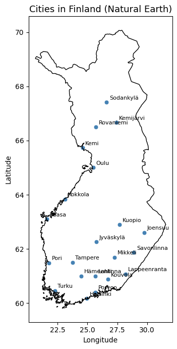
3. Static map with Matplotlib + GeoPandas#

In this section, we draw Finland’s country border and overlay populated places. City names are added as annotations to make the map easier to read.

import matplotlib.pyplot as plt

fig, ax = plt.subplots(figsize=(5, 7))

# Draw Finland's border
finland_border = countries[countries["ADM0_A3"] == "FIN"]
finland_border.boundary.plot(ax=ax, color="black", linewidth=1)

finland.plot(
    ax=ax,
    color="steelblue",
    markersize=40,
    edgecolor="white",
    linewidth=0.5,
)

# Label each city
for _, row in finland.iterrows():
    ax.annotate(
        row["name"],
        xy=(row.geometry.x, row.geometry.y),
        xytext=(4, 4),
        textcoords="offset points",
        fontsize=8,
    )

ax.set_title("Cities in Finland (Natural Earth)", fontsize=13)
ax.set_xlabel("Longitude")
ax.set_ylabel("Latitude")
plt.tight_layout()
plt.show()

../_images/54398b73b249070b9ae51bcbd4240e7e77a9a6a7a71c526ecd36fc907fda6f31.png

4. Interactive map with Folium#

Finally, we create a web map centered on Austria. We add the Austria border as a GeoJSON layer and draw one circle marker per Austrian city with a popup and tooltip.

import folium

# Create a map centred on Austria using CartoDB Positron as the only basemap
m = folium.Map(
    location=[47.5, 14.5],
    zoom_start=7,
    tiles="CartoDB positron",
)

# Add Austria border as a GeoJSON layer
austria_border = countries[countries["ADM0_A3"] == "AUT"]
folium.GeoJson(
    data=austria_border.__geo_interface__,
    style_function=lambda _: {
        "fillColor": "lightyellow",
        "color": "black",
        "weight": 2,
        "fillOpacity": 0.25,
    },
    name="Austria border",
).add_to(m)

# Add one CircleMarker per Austrian city
for _, row in austria.iterrows():
    is_capital = row["name"] == "Vienna"
    folium.CircleMarker(
        location=[row.geometry.y, row.geometry.x],
        radius=6 if is_capital else 4,
        color="steelblue",
        fill=True,
        fill_opacity=0.8,
        tooltip=row["name"],
    ).add_to(m)

# Fit view to Austria boundary
bounds = austria_border.total_bounds  # minx, miny, maxx, maxy
m.fit_bounds([[bounds[1], bounds[0]], [bounds[3], bounds[2]]])

m

Make this Notebook Trusted to load map: File -> Trust Notebook

Tutorial 1: Introduction to Python and Jupyter

Contents