Lecture 4 - Deep Learning Tutorial Notebook: Pool Detection with YOLO

Attention

Students are encouraged to use the CSC Mahti platform.

What we’re going to cover

In this notebook, we follow an end-to-end object detection workflow on an Aerial Imagery and OSM (OpenStreetMap) swimming pool data.

We’ll use the region of Galicia (Spain) for training and Viana do Castelo (Portugal) for validation.

We’re going to cover in this tutorial:

Topic	Contents
0. Computer vision libraries for YOLO	We’ll set up the Ultralytics and Supervision libraries to handle our object detection tasks.
1. Download and prepare data	We’ll pull dataset files from Hugging Face and build a standard YOLO dataset configuration.
2. Model 0: Train a local baseline	We’ll train a small, lightweight YOLO model (yolo11n) for a few epochs to establish a baseline.
3. Model 1: Load a pretrained reference model	We’ll load Mozilla.ai’s fully trained pool detector for a teaching comparison.
4. Validate and compare predictions	Let’s evaluate both models on the same validation split and inspect their predictions side-by-side.
5. The Graz Test (Out-of-domain evaluation)	We’ll run qualitative tests on un-seen Graz tiles to discuss transferability and failure modes.

Notes for interpretation

• This is a teaching comparison. The two models differ in size and training history.

• OSM-derived labels can be incomplete or noisy, so qualitative checks are part of the learning process.

• Results on the Graz tiles are out-of-domain and should be read as behavior checks, not benchmark scores.

Reference model: https://huggingface.co/mozilla-ai/swimming-pool-detector

What we will cover:

First, let’s make sure we have all the necessary packages installed:

%pip install -q ultralytics supervision rasterio datasets huggingface_hub

     ━━━━━━━━━━━━━━━━━━━━━━━━━━━━━━━━━━━━━━━━ 41.9/41.9 kB 3.9 MB/s eta 0:00:00
   ━━━━━━━━━━━━━━━━━━━━━━━━━━━━━━━━━━━━━━━━ 1.2/1.2 MB 48.5 MB/s eta 0:00:00
   ━━━━━━━━━━━━━━━━━━━━━━━━━━━━━━━━━━━━━━━━ 217.4/217.4 kB 23.9 MB/s eta 0:00:00
?25h

0. Setup Libraries and Verify Environment

What are Ultralytics and Supervision?

• Ultralytics is the library behind YOLO (You Only Look Once), a state-of-the-art, real-time object detection system. We’ll use it to train and evaluate our models.

• Supervision is a highly useful computer vision utility library that makes writing filtering, tracking, and annotation code much easier.

Let’s import everything we need and print out our key version information so our runs are reproducible and easier to debug.

import random
import shutil
import zipfile
from pathlib import Path

import datasets
import numpy as np
import supervision as sv
import torch
import ultralytics
from huggingface_hub import hf_hub_download
from ultralytics import YOLO

# Set random seeds for reproducibility across Python, NumPy, and PyTorch.
# Ultralytics' train(seed=...) handles its own internal seeding on top of this.
SEED = 42
random.seed(SEED)
np.random.seed(SEED)
torch.manual_seed(SEED)
if torch.cuda.is_available():
    torch.cuda.manual_seed_all(SEED)

# Check versions
print(f"Ultralytics version: {ultralytics.__version__}")
print(f"Supervision version: {sv.__version__}")
print(f"Datasets version: {datasets.__version__}")
print(f"PyTorch version: {torch.__version__}")

Creating new Ultralytics Settings v0.0.6 file ✅ 
View Ultralytics Settings with 'yolo settings' or at '/root/.config/Ultralytics/settings.json'
Update Settings with 'yolo settings key=value', i.e. 'yolo settings runs_dir=path/to/dir'. For help see https://docs.ultralytics.com/quickstart/#ultralytics-settings.
Ultralytics version: 8.4.40
Supervision version: 0.27.0.post2
Datasets version: 4.0.0
PyTorch version: 2.10.0+cu128
Seed: 42

1. Getting and preparing the dataset

We’re going to use an OSM Swimming Pools dataset.

Instead of writing complex download scripts from scratch, we’ll pull the training split, validation split, and YOLO configuration directly from Hugging Face using hf_hub_download.

So what is Hugging Face?

Hugging Face is pretty much the GitHub for machine learning.

It’s a platform where developers, organizations, and enthusiasts collaborate by uploading and distributing three types of assets:

• Models — pretrained models that can be downloaded for immediate use or fine-tuning to fit your data. This is how mozilla-ai/swimming-pool-detector was created.

• Datasets — prepared datasets that can be utilized directly, usually split into training and evaluation parts. This is where mozilla-ai/osm-swimming-pools comes from.

• Spaces — miniature apps that allow users to interact with a trained model via a web browser without any installations.

Why does this matter for us?

1. Reproducibility. Each model / dataset is associated with a project repo_id (e.g. mozilla-ai/osm-swimming-pools) to store it.

2. Caching. When you download a file for the first time it goes to ~/. cache/huggingface/. The second time, it’s instant.

3. Versioning. The repos are git-based under the hood

4. Ecosystem. A lot of libraries like transformers, datasets, etc…

Think of it like: instead of training a model from scratch every time, you have one central place where the community puts its work. You pull what you need, build on top of it, and (if you want) push your own contributions back.

In our case, this saved us from manually collecting aerial imagery of swimming pools across Galicia and from training a large YOLO model for days.
Both already existed on the Hub; we just borrowed them.

1.1 Building the YOLO configuration

YOLO models require data to be organized in a certain format, often specified by a .yaml file.
This file indicates where the training images are, where the validation images are, and which classes we want to predict.

We will download the zip files, extract them safely and create our local yolo_dataset.yaml.

DATA_DIR = Path("osm_pools_dataset")
DATA_DIR.mkdir(exist_ok=True)

# Download the necessary files
for filename in ["train.zip", "val.zip", "yolo_dataset.yaml"]:
    local = hf_hub_download(
        repo_id="mozilla-ai/osm-swimming-pools",
        repo_type="dataset",
        filename=filename,
    )
    target = DATA_DIR / filename
    if not target.exists():
        shutil.copy(local, target)

# Idempotent extraction: only unzip if expected split folders are missing.
if not (DATA_DIR / "Galicia").exists() or not (DATA_DIR / "Viana do Castelo").exists():
    for zip_name in ["train.zip", "val.zip"]:
        with zipfile.ZipFile(DATA_DIR / zip_name) as zf:
            zf.extractall(DATA_DIR)

galicia = next(DATA_DIR.rglob("Galicia"))
viana = next(DATA_DIR.rglob("Viana do Castelo"))

# Create the YAML configuration file for YOLO
yaml_path = DATA_DIR / "yolo_dataset.yaml"
yaml_path.write_text(
    f"path: {galicia.parent.resolve()}\n"
    f"train: Galicia\n"
    f"val: Viana do Castelo\n"
    f"\n"
    f"names:\n"
    f"  0: swimming_pool\n",
    encoding="utf-8",
)
print(f" Train: {galicia} \n Val: {viana}")

UserWarning: 
Error while fetching `HF_TOKEN` secret value from your vault: 'Requesting secret HF_TOKEN timed out. Secrets can only be fetched when running from the Colab UI.'.
You are not authenticated with the Hugging Face Hub in this notebook.
If the error persists, please let us know by opening an issue on GitHub (https://github.com/huggingface/huggingface_hub/issues/new).

Warning: You are sending unauthenticated requests to the HF Hub. Please set a HF_TOKEN to enable higher rate limits and faster downloads.
WARNING:huggingface_hub.utils._http:Warning: You are sending unauthenticated requests to the HF Hub. Please set a HF_TOKEN to enable higher rate limits and faster downloads.

 Train: osm_pools_dataset/datasets/Galicia 
 Val: osm_pools_dataset/datasets/Viana do Castelo

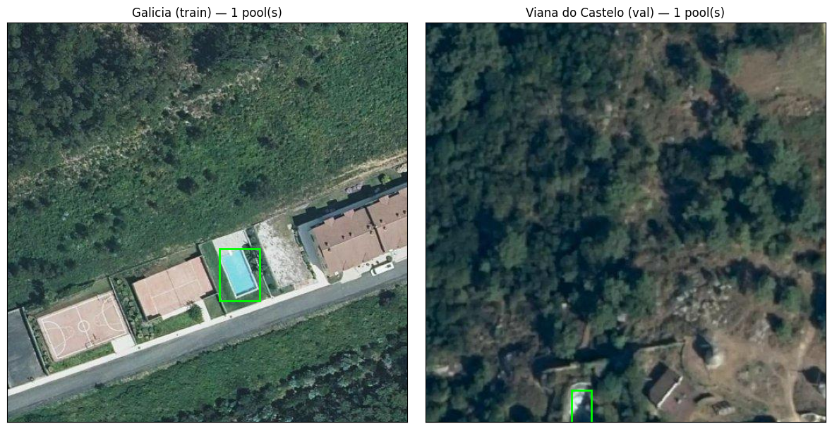
1.2 Understanding the downloaded dataset

The Hugging Face download provides a small but realistic aerial-object-detection dataset:

• Two geographic areas: Galicia for training and Viana do Castelo for validation.

• One class: swimming_pool.

• Each image is a high-resolution aerial tile with a corresponding YOLO label file.

• Labels are stored as normalized center-x, center-y, width, and height values

import matplotlib.patches as patches
import matplotlib.pyplot as plt
from PIL import Image


def read_yolo_labels(label_path: Path):
    # Read a YOLO label file. Returns a list of (class_id, cx, cy, w, h) tuples.
    if not label_path.exists():
        return []
    rows = []
    for line in label_path.read_text().splitlines():
        parts = line.strip().split()
        if len(parts) >= 5:
            cls, cx, cy, w, h = parts[:5]
            rows.append((int(cls), float(cx), float(cy), float(w), float(h)))
    return rows


def first_image_with_labels(images_dir: Path):
    # Find the first image in a split folder that actually has a non-empty label file.
    img_dir = images_dir / "images" if (images_dir / "images").exists() else images_dir
    lbl_dir = images_dir / "labels" if (images_dir / "labels").exists() else images_dir
    for img_path in sorted(img_dir.glob("*.jpg")) + sorted(img_dir.glob("*.png")):
        label_path = lbl_dir / (img_path.stem + ".txt")
        rows = read_yolo_labels(label_path)
        if rows:
            return img_path, rows
    # Fall back to the first image even if it has no labels.
    any_img = next(
        iter(sorted(img_dir.glob("*.jpg")) + sorted(img_dir.glob("*.png"))), None
    )
    return any_img, []


fig, axes = plt.subplots(1, 2, figsize=(12, 6))
for ax, split_dir, title in [
    (axes[0], galicia, "Galicia (train)"),
    (axes[1], viana, "Viana do Castelo (val)"),
]:
    img_path, rows = first_image_with_labels(split_dir)
    if img_path is None:
        ax.set_title(f"{title}: no images found")
        ax.axis("off")
        continue
    image = Image.open(img_path)
    w, h = image.size
    ax.imshow(image)
    for _, cx, cy, bw, bh in rows:
        x = (cx - bw / 2) * w
        y = (cy - bh / 2) * h
        rect = patches.Rectangle(
            (x, y),
            bw * w,
            bh * h,
            linewidth=2,
            edgecolor="lime",
            facecolor="none",
        )
        ax.add_patch(rect)
    ax.set_title(f"{title} — {len(rows)} pool(s)")
    ax.set_xticks([])
    ax.set_yticks([])

plt.tight_layout()
plt.show()

2. Model 0: Build a baseline model (yolo11n)

It’s time to build a baseline model.

A baseline is a simpler, smaller model we create as a starting point. We use it to ensure our pipeline works before moving on to larger, more complex models.

We’ll train a compact model (yolo11n.pt, where ‘n’ stands for nano) for just a few epochs to keep training manageable.

We need to set the following parameters:

• data - the path to the YAML file we just created.

• epochs - the number of times the model will see the entire dataset.

• imgsz - the resolution we are resizing the images to for training.

• batch - the number of samples processed before the model updates its internal parameters.

EPOCHS = 3

# Instantiate the baseline model
own_model = YOLO("yolo11n.pt")

# Train the model
train_results = own_model.train(
    data=str(yaml_path),
    epochs=EPOCHS,
    imgsz=512,
    batch=16,
    seed=SEED,
    project="runs/detect_teaching",
    name="own_pool_detector",
    exist_ok=True,
    plots=True,
)

# Safely capture the best weights for later use
OWN_WEIGHTS = Path(train_results.save_dir) / "weights" / "best.pt"
if not OWN_WEIGHTS.exists():
    raise FileNotFoundError(f"Expected checkpoint not found: {OWN_WEIGHTS}")

print(f"\nOwn model weights saved to: {OWN_WEIGHTS}")

Downloading https://github.com/ultralytics/assets/releases/download/v8.4.0/yolo11n.pt to 'yolo11n.pt': 100% ━━━━━━━━━━━━ 5.4MB 92.7MB/s 0.1s
Ultralytics 8.4.40 🚀 Python-3.12.13 torch-2.10.0+cu128 CUDA:0 (Tesla T4, 14913MiB)
engine/trainer: agnostic_nms=False, amp=True, angle=1.0, augment=False, auto_augment=randaugment, batch=16, bgr=0.0, box=7.5, cache=False, cfg=None, classes=None, close_mosaic=10, cls=0.5, cls_pw=0.0, compile=False, conf=None, copy_paste=0.0, copy_paste_mode=flip, cos_lr=False, cutmix=0.0, data=osm_pools_dataset/yolo_dataset.yaml, degrees=0.0, deterministic=True, device=None, dfl=1.5, dnn=False, dropout=0.0, dynamic=False, embed=None, end2end=None, epochs=3, erasing=0.4, exist_ok=True, fliplr=0.5, flipud=0.0, format=torchscript, fraction=1.0, freeze=None, half=False, hsv_h=0.015, hsv_s=0.7, hsv_v=0.4, imgsz=512, int8=False, iou=0.7, keras=False, kobj=1.0, line_width=None, lr0=0.01, lrf=0.01, mask_ratio=4, max_det=300, mixup=0.0, mode=train, model=yolo11n.pt, momentum=0.937, mosaic=1.0, multi_scale=0.0, name=own_pool_detector, nbs=64, nms=False, opset=None, optimize=False, optimizer=auto, overlap_mask=True, patience=100, perspective=0.0, plots=True, pose=12.0, pretrained=True, profile=False, project=runs/detect_teaching, rect=False, resume=False, retina_masks=False, rle=1.0, save=True, save_conf=False, save_crop=False, save_dir=/content/runs/detect/runs/detect_teaching/own_pool_detector, save_frames=False, save_json=False, save_period=-1, save_txt=False, scale=0.5, seed=42, shear=0.0, show=False, show_boxes=True, show_conf=True, show_labels=True, simplify=True, single_cls=False, source=None, split=val, stream_buffer=False, task=detect, time=None, tracker=botsort.yaml, translate=0.1, val=True, verbose=True, vid_stride=1, visualize=False, warmup_bias_lr=0.1, warmup_epochs=3.0, warmup_momentum=0.8, weight_decay=0.0005, workers=8, workspace=None
Downloading https://ultralytics.com/assets/Arial.ttf to '/root/.config/Ultralytics/Arial.ttf': 100% ━━━━━━━━━━━━ 755.1KB 41.8MB/s 0.0s
Overriding model.yaml nc=80 with nc=1

                   from  n    params  module                                       arguments                     
  0                  -1  1       464  ultralytics.nn.modules.conv.Conv             [3, 16, 3, 2]                 
  1                  -1  1      4672  ultralytics.nn.modules.conv.Conv             [16, 32, 3, 2]                
  2                  -1  1      6640  ultralytics.nn.modules.block.C3k2            [32, 64, 1, False, 0.25]      
  3                  -1  1     36992  ultralytics.nn.modules.conv.Conv             [64, 64, 3, 2]                
  4                  -1  1     26080  ultralytics.nn.modules.block.C3k2            [64, 128, 1, False, 0.25]     
  5                  -1  1    147712  ultralytics.nn.modules.conv.Conv             [128, 128, 3, 2]              
  6                  -1  1     87040  ultralytics.nn.modules.block.C3k2            [128, 128, 1, True]           
  7                  -1  1    295424  ultralytics.nn.modules.conv.Conv             [128, 256, 3, 2]              
  8                  -1  1    346112  ultralytics.nn.modules.block.C3k2            [256, 256, 1, True]           
  9                  -1  1    164608  ultralytics.nn.modules.block.SPPF            [256, 256, 5]                 
 10                  -1  1    249728  ultralytics.nn.modules.block.C2PSA           [256, 256, 1]                 
 11                  -1  1         0  torch.nn.modules.upsampling.Upsample         [None, 2, 'nearest']          
 12             [-1, 6]  1         0  ultralytics.nn.modules.conv.Concat           [1]                           
 13                  -1  1    111296  ultralytics.nn.modules.block.C3k2            [384, 128, 1, False]          
 14                  -1  1         0  torch.nn.modules.upsampling.Upsample         [None, 2, 'nearest']          
 15             [-1, 4]  1         0  ultralytics.nn.modules.conv.Concat           [1]                           
 16                  -1  1     32096  ultralytics.nn.modules.block.C3k2            [256, 64, 1, False]           
 17                  -1  1     36992  ultralytics.nn.modules.conv.Conv             [64, 64, 3, 2]                
 18            [-1, 13]  1         0  ultralytics.nn.modules.conv.Concat           [1]                           
 19                  -1  1     86720  ultralytics.nn.modules.block.C3k2            [192, 128, 1, False]          
 20                  -1  1    147712  ultralytics.nn.modules.conv.Conv             [128, 128, 3, 2]              
 21            [-1, 10]  1         0  ultralytics.nn.modules.conv.Concat           [1]                           
 22                  -1  1    378880  ultralytics.nn.modules.block.C3k2            [384, 256, 1, True]           
 23        [16, 19, 22]  1    430867  ultralytics.nn.modules.head.Detect           [1, 16, None, [64, 128, 256]] 
YOLO11n summary: 182 layers, 2,590,035 parameters, 2,590,019 gradients, 6.4 GFLOPs

Transferred 448/499 items from pretrained weights
Freezing layer 'model.23.dfl.conv.weight'
AMP: running Automatic Mixed Precision (AMP) checks...
Downloading https://github.com/ultralytics/assets/releases/download/v8.4.0/yolo26n.pt to 'yolo26n.pt': 100% ━━━━━━━━━━━━ 5.3MB 133.6MB/s 0.0s
AMP: checks passed ✅
train: Fast image access ✅ (ping: 0.0±0.0 ms, read: 1366.7±594.6 MB/s, size: 71.2 KB)
train: Scanning /content/osm_pools_dataset/datasets/Galicia... 6913 images, 0 backgrounds, 0 corrupt: 100% ━━━━━━━━━━━━ 6913/6913 2.4Kit/s 2.9s0.0s
train: New cache created: /content/osm_pools_dataset/datasets/Galicia.cache
albumentations: Blur(p=0.01, blur_limit=(3, 7)), MedianBlur(p=0.01, blur_limit=(3, 7)), ToGray(p=0.01, method='weighted_average', num_output_channels=3), CLAHE(p=0.01, clip_limit=(1.0, 4.0), tile_grid_size=(8, 8))
val: Fast image access ✅ (ping: 0.0±0.0 ms, read: 774.2±563.8 MB/s, size: 44.8 KB)
val: Scanning /content/osm_pools_dataset/datasets/Viana do Castelo... 455 images, 0 backgrounds, 0 corrupt: 100% ━━━━━━━━━━━━ 455/455 1.2Kit/s 0.4s<0.1s
val: New cache created: /content/osm_pools_dataset/datasets/Viana do Castelo.cache
optimizer: 'optimizer=auto' found, ignoring 'lr0=0.01' and 'momentum=0.937' and determining best 'optimizer', 'lr0' and 'momentum' automatically... 
optimizer: AdamW(lr=0.002, momentum=0.9) with parameter groups 81 weight(decay=0.0), 88 weight(decay=0.0005), 87 bias(decay=0.0)
Plotting labels to /content/runs/detect/runs/detect_teaching/own_pool_detector/labels.jpg... 
Image sizes 512 train, 512 val
Using 2 dataloader workers
Logging results to /content/runs/detect/runs/detect_teaching/own_pool_detector
Starting training for 3 epochs...

      Epoch    GPU_mem   box_loss   cls_loss   dfl_loss  Instances       Size
        1/3      1.39G      2.056      2.273      1.346          2        512: 100% ━━━━━━━━━━━━ 433/433 3.5it/s 2:02<0.3ss
                 Class     Images  Instances      Box(P          R      mAP50  mAP50-95): 100% ━━━━━━━━━━━━ 15/15 1.4it/s 10.6s.2s
                   all        455        540      0.709      0.712      0.704      0.327

      Epoch    GPU_mem   box_loss   cls_loss   dfl_loss  Instances       Size
        2/3      1.64G      1.995      1.547      1.304          1        512: 100% ━━━━━━━━━━━━ 433/433 4.4it/s 1:38<0.2ss
                 Class     Images  Instances      Box(P          R      mAP50  mAP50-95): 100% ━━━━━━━━━━━━ 15/15 5.6it/s 2.7s0.2s
                   all        455        540      0.782      0.706      0.728      0.345

      Epoch    GPU_mem   box_loss   cls_loss   dfl_loss  Instances       Size
        3/3      1.64G      1.942       1.39      1.279          8        512: 100% ━━━━━━━━━━━━ 433/433 4.4it/s 1:38<0.2ss
                 Class     Images  Instances      Box(P          R      mAP50  mAP50-95): 100% ━━━━━━━━━━━━ 15/15 5.6it/s 2.7s0.2s
                   all        455        540      0.789      0.757      0.763      0.368

3 epochs completed in 0.093 hours.
Optimizer stripped from /content/runs/detect/runs/detect_teaching/own_pool_detector/weights/last.pt, 5.4MB
Optimizer stripped from /content/runs/detect/runs/detect_teaching/own_pool_detector/weights/best.pt, 5.4MB

Validating /content/runs/detect/runs/detect_teaching/own_pool_detector/weights/best.pt...
Ultralytics 8.4.40 🚀 Python-3.12.13 torch-2.10.0+cu128 CUDA:0 (Tesla T4, 14913MiB)
YOLO11n summary (fused): 101 layers, 2,582,347 parameters, 0 gradients, 6.3 GFLOPs
                 Class     Images  Instances      Box(P          R      mAP50  mAP50-95): 100% ━━━━━━━━━━━━ 15/15 3.1it/s 4.9s0.3s
                   all        455        540      0.791      0.757      0.763      0.368
Speed: 0.2ms preprocess, 2.0ms inference, 0.0ms loss, 2.2ms postprocess per image
Results saved to /content/runs/detect/runs/detect_teaching/own_pool_detector

Own model weights saved to: /content/runs/detect/runs/detect_teaching/own_pool_detector/weights/best.pt

3. Model 1: Load the pretrained reference model

We now have a baseline but what happens if we use a model that has been trained for much longer, on more data, with a slightly larger architecture?

Instead of training a massive model from scratch, we can load a pretrained model. This is a common practice in machine learning: finding a model architecture that works for a similar problem and utilizing its learned weights.

So now load the Mozilla.ai model and reload our own trained weights so we can compare them side-by-side.

from huggingface_hub import hf_hub_download
from ultralytics import YOLO


def load_pretrained_yolo(repo_id: str, filename: str = "model.pt") -> YOLO:
    """Helper function to download and load a model from Hugging Face."""
    weights_path = hf_hub_download(repo_id=repo_id, filename=filename)
    return YOLO(weights_path)


# Load both models
pretrained_model = load_pretrained_yolo("mozilla-ai/swimming-pool-detector")
own_model = YOLO(str(OWN_WEIGHTS))

# Always a good idea to check class mappings!
print(f"Pretrained model classes: {pretrained_model.names}")
print(f"Own model classes:        {own_model.names}")

Pretrained model classes: {0: 'swimming_pool'}
Own model classes:        {0: 'swimming_pool'}

4. Validate both models and compare outputs

Now that both models are loaded, we evaluate them on the same validation split (Viana do Castelo).

4.1 Setup evaluation metrics

For object detection, instead of pure accuracy, we typically look at mAP (mean Average Precision).

• mAP@0.5 measures precision when the predicted bounding box overlaps the ground truth by at least 50%.

• mAP@0.5:0.95 is a stricter metric that averages the precision across multiple overlap thresholds.

from pathlib import Path

import matplotlib.pyplot as plt
import numpy as np
import supervision as sv
from datasets import load_dataset

DATA_DIR = Path("osm_pools_dataset")
yaml_path = DATA_DIR / "yolo_dataset.yaml"

own_arch = Path(own_model.ckpt_path).stem if own_model.ckpt_path else "unknown"
pro_arch = (
    Path(pretrained_model.ckpt_path).stem if pretrained_model.ckpt_path else "unknown"
)

print(f"--- Own model ({own_arch}, {EPOCHS} epochs) ---")
own_metrics = own_model.val(data=str(yaml_path), imgsz=512, conf=0.25)

print(f"\n--- Mozilla.ai model ({pro_arch}, fully trained) ---")
pro_metrics = pretrained_model.val(data=str(yaml_path), imgsz=512, conf=0.25)

print("\n=== Summary (teaching comparison) ===")
print(
    f"Own      mAP@0.5: {own_metrics.box.map50:.3f} | mAP@0.5:0.95: {own_metrics.box.map:.3f}"
)
print(
    f"Mozilla  mAP@0.5: {pro_metrics.box.map50:.3f} | mAP@0.5:0.95: {pro_metrics.box.map:.3f}"
)

--- Own model (best, 3 epochs) ---
Ultralytics 8.4.40 🚀 Python-3.12.13 torch-2.10.0+cu128 CUDA:0 (Tesla T4, 14913MiB)
YOLO11n summary (fused): 101 layers, 2,582,347 parameters, 0 gradients, 6.3 GFLOPs
val: Fast image access ✅ (ping: 0.0±0.0 ms, read: 1264.8±337.3 MB/s, size: 42.5 KB)
val: Scanning /content/osm_pools_dataset/datasets/Viana do Castelo.cache... 455 images, 0 backgrounds, 0 corrupt: 100% ━━━━━━━━━━━━ 455/455 190.8Mit/s 0.0s
                 Class     Images  Instances      Box(P          R      mAP50  mAP50-95): 100% ━━━━━━━━━━━━ 29/29 6.3it/s 4.6s0.1s
                   all        455        540      0.785      0.756      0.742      0.354
Speed: 1.5ms preprocess, 3.0ms inference, 0.0ms loss, 1.2ms postprocess per image
Results saved to /content/runs/detect/val

--- Mozilla.ai model (model, fully trained) ---
Ultralytics 8.4.40 🚀 Python-3.12.13 torch-2.10.0+cu128 CUDA:0 (Tesla T4, 14913MiB)
YOLO11m summary (fused): 125 layers, 20,030,803 parameters, 0 gradients, 67.6 GFLOPs
val: Fast image access ✅ (ping: 0.0±0.0 ms, read: 1842.1±700.9 MB/s, size: 43.3 KB)
val: Scanning /content/osm_pools_dataset/datasets/Viana do Castelo.cache... 455 images, 0 backgrounds, 0 corrupt: 100% ━━━━━━━━━━━━ 455/455 212.0Mit/s 0.0s
                 Class     Images  Instances      Box(P          R      mAP50  mAP50-95): 100% ━━━━━━━━━━━━ 29/29 2.9it/s 10.0s.3s
                   all        455        540       0.82      0.748        0.7      0.368
Speed: 1.1ms preprocess, 16.8ms inference, 0.0ms loss, 1.2ms postprocess per image
Results saved to /content/runs/detect/val-2

=== Summary (teaching comparison) ===
Own      mAP@0.5: 0.742 | mAP@0.5:0.95: 0.354
Mozilla  mAP@0.5: 0.700 | mAP@0.5:0.95: 0.368

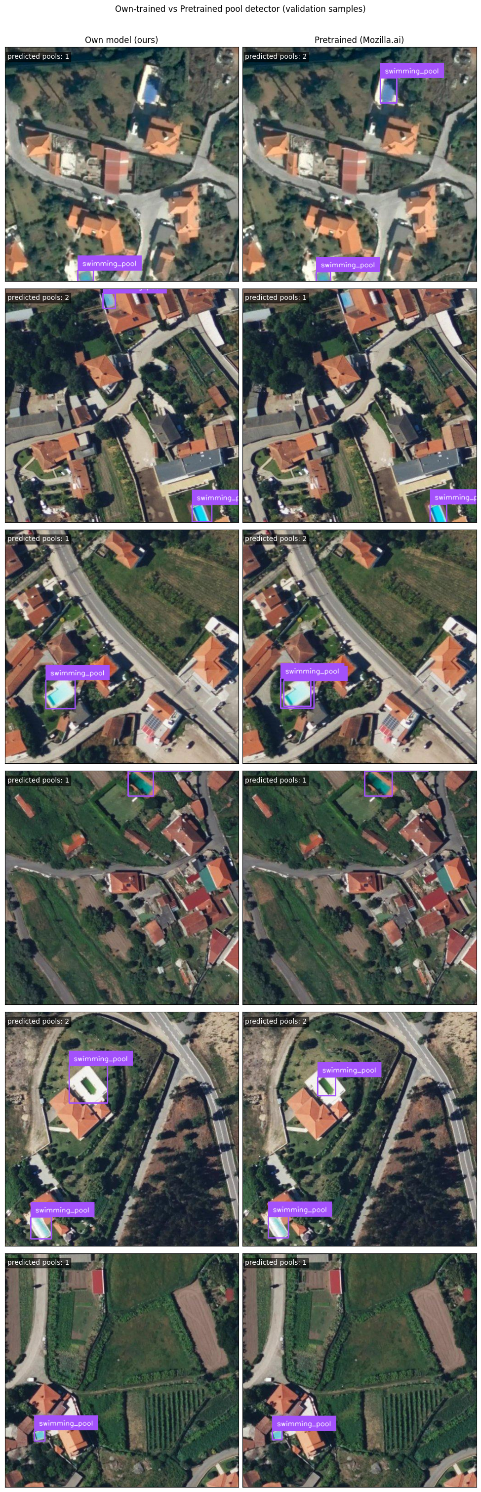
4.2 Visualizing the predictions

Numeric metrics like mAP are great, but since we’re dealing with image data, let’s plot them.

First, we inspect side-by-side the predictions. This helps connect our numeric metrics with actual visual model behavior.

Does the baseline miss smaller pools? Does it hallucinate pools where there are none?

# Load the validation dataset directly to grab sample images
ds = load_dataset("mozilla-ai/osm-swimming-pools", split="validation")
if len(ds) == 0:
    raise ValueError("Validation split is empty.")

# Set up Supervision annotators
box_annotator = sv.BoxAnnotator()
label_annotator = sv.LabelAnnotator()

# Pick a few random samples
sample_count = min(6, len(ds))
rng = np.random.default_rng(SEED)
sample_indices = sorted(rng.choice(len(ds), size=sample_count, replace=False).tolist())

# Plot predictions
fig, axes = plt.subplots(sample_count, 2, figsize=(10, 5 * sample_count))
if sample_count == 1:
    axes = np.expand_dims(axes, axis=0)

axes[0, 0].set_title("Own model (ours)", fontsize=12)
axes[0, 1].set_title("Pretrained (Mozilla.ai)", fontsize=12)

for row, ds_i in enumerate(sample_indices):
    image = ds[ds_i]["image"]

    for col, m in enumerate([own_model, pretrained_model]):
        # Make predictions
        result = m.predict(image, conf=0.25, verbose=False)[0]

        # Convert Ultralytics results to Supervision detections for easy plotting
        detections = sv.Detections.from_ultralytics(result)
        annotated = box_annotator.annotate(scene=image.copy(), detections=detections)
        annotated = label_annotator.annotate(scene=annotated, detections=detections)

        # Show the image
        axes[row, col].imshow(annotated)
        axes[row, col].set_xticks([])
        axes[row, col].set_yticks([])
        axes[row, col].text(
            5,
            25,
            f"predicted pools: {len(detections)}",
            color="white",
            fontsize=10,
            bbox=dict(facecolor="black", alpha=0.6, pad=2),
        )

plt.suptitle("Own-trained vs Pretrained pool detector (validation samples)", y=1.005)
plt.tight_layout()
plt.show()

5. The Graz Test (Evaluating on out-of-domain data)

Something to be aware of in machine learning is generalization.

Does our model only know how to find pools in Galicia and Viana do Castelo? Or has it learned the general concept of a pool well enough to find them anywhere in the world?

We are going to test on tiles from Graz, Austria.

Because Graz is geographically distinct from our training data, we call this out-of-domain testing.

But keep in mind:

• Detection counts here are not benchmark metrics.

• We use this to discuss transferability, false positives (predicting a pool where there isn’t one), and false negatives (missing an actual pool).

Note: tiles.zip is required !!

Place tiles.zip in the project root (the directory containing pyproject.toml) before running the next cell. The next cell checks for tiles.zip and unzips it automatically if the tiles/ directory is not present.

from pathlib import Path
import zipfile

TILES_ZIP = Path("tiles.zip")
TILES_DIR = Path("tiles")

if not TILES_ZIP.exists():
    raise FileNotFoundError(f"Missing archive: {TILES_ZIP.resolve()}")

if TILES_DIR.exists():
    print(f"Tiles already extracted: {TILES_DIR}")
else:
    with zipfile.ZipFile(TILES_ZIP) as zf:
        zf.extractall(".")
    print(f"Extracted {TILES_ZIP} -> {TILES_DIR}")

Tiles already extracted: tiles

from pathlib import Path
import matplotlib.pyplot as plt
import supervision as sv

CONF = 0.2
TILE_NAMES = [
    "18_142309_92193.jpg",
    "18_142308_92186.jpg",
    "18_142302_92189.jpg",
    "18_142297_92185.jpg",
]
PROVIDERS = {
    "Basemap": Path("tiles/basemap_at"),
    "Mapbox": Path("tiles/mapbox"),
}

# Validate up front so failures are loud and specific.
missing = [
    f"{provider}:{name}"
    for provider, directory in PROVIDERS.items()
    for name in TILE_NAMES
    if not (directory / name).exists()
]
if missing:
    raise FileNotFoundError("Missing tiles: " + ", ".join(missing))

box_annotator = sv.BoxAnnotator()
label_annotator = sv.LabelAnnotator()

fig, axes = plt.subplots(
    len(TILE_NAMES), len(PROVIDERS), figsize=(14, 4 * len(TILE_NAMES))
)

for row, name in enumerate(TILE_NAMES):
    for col, (provider, directory) in enumerate(PROVIDERS.items()):
        image_path = directory / name
        result = pretrained_model.predict(
            source=str(image_path), conf=CONF, verbose=False
        )[0]
        detections = sv.Detections.from_ultralytics(result)

        scene = plt.imread(image_path).copy()
        scene = box_annotator.annotate(scene=scene, detections=detections)
        scene = label_annotator.annotate(
            scene=scene,
            detections=detections,
            labels=[f"pool {c:.2f}" for c in detections.confidence],
        )

        ax = axes[row, col]
        ax.imshow(scene)
        ax.set_title(
            f"{name} | {provider} | detections: {len(detections)}", fontsize=10
        )
        ax.set_xticks([])
        ax.set_yticks([])

plt.suptitle("Fixed Graz tiles: Basemap (left) vs Mapbox (right)", y=1.001)
plt.tight_layout()
plt.show()

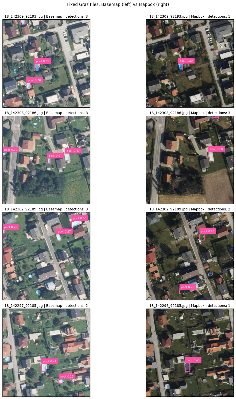
Why compare two imagery providers?

Pool detection performance depends heavily on the input imagery, not just the model. Running the same model on tiles from two independent providers lets us separate model behaviour from imagery characteristics.

What we learn from this comparison ? What are the differences in pool detection performance between the two imagery providers? Are there specific types of pools or environments where one provider’s imagery leads to better detection than the other?